


The official site for annual CO2 is Mauna Loa. The station at 11,300 feet high (3,444 meters), has a 131-foot (40-meter) tower that collects air to measure levels of carbon dioxide.
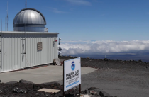
In 1958, Charles Keeling choose to install an atmospheric carbon dioxide monitoring system on Mauna Loa, a volcanic peak on the Big Island of Hawaii as the remote location would allow only carbon dioxide that had mixed with the atmosphere to be measured.
The latest annual numbers are around 420 which averages 0.04% of the air. Levels are lowest during July as vegetation is using it in photosynthesis and releasing O2.
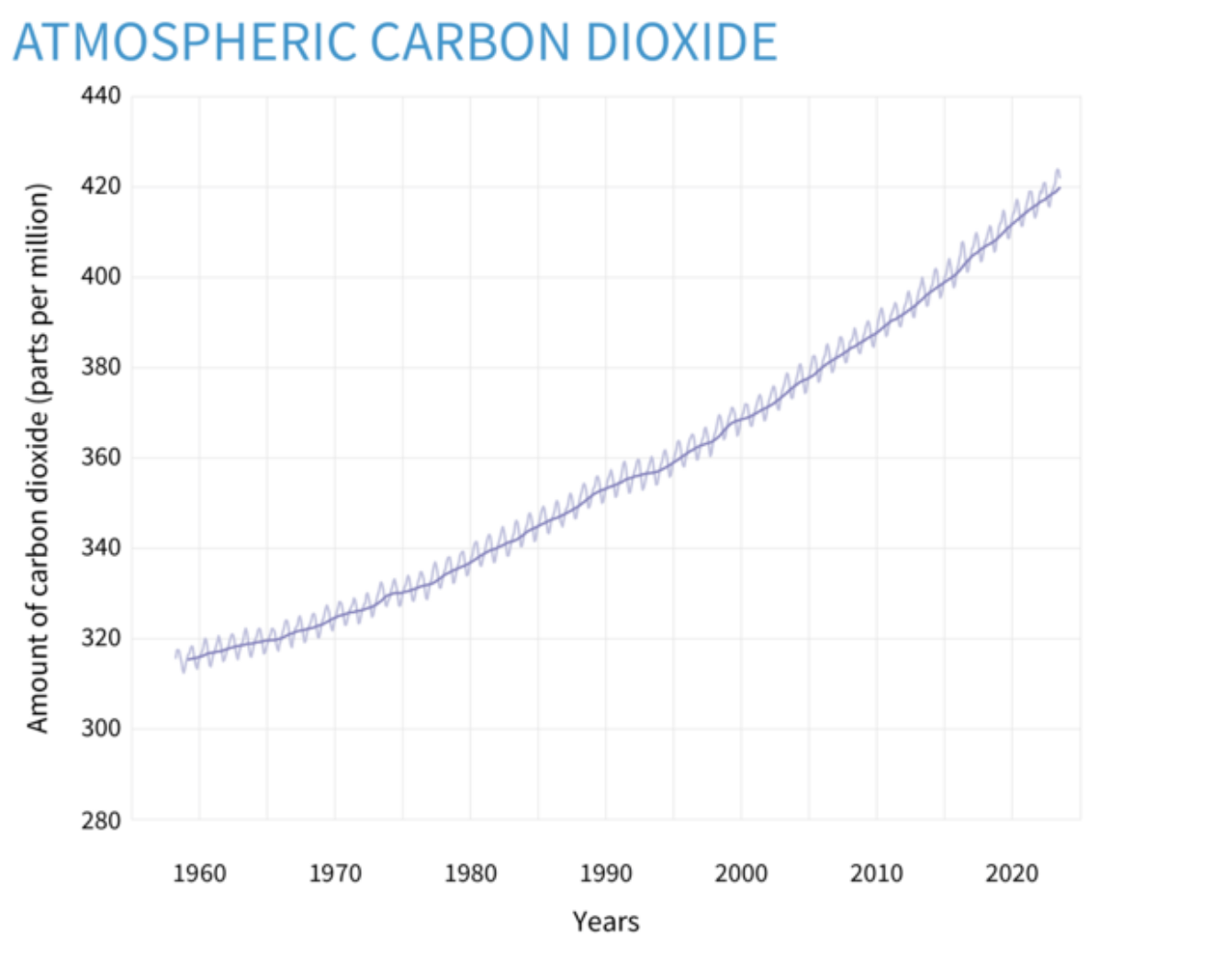
It varies greatly where we actually live because when we breathe in the air with just 0.04% (420) ppm CO2), when we breathe out, we release 42,000 ppm. CO2 levels are much higher in populated areas and especially when people congregate (churches, schools, restaurants. even you home when the family and pets are there).
ITS NOT POLLUTION
HOME AND OFFICE AND SCHOOLS
Levels exceeding 2000 ppm are found in small offices and Ken. C., a science teacher writes, “In one classroom of 30 students after lunch reached CO2 levels of 4,825 ppm with the door closed. According to ASHRAE, the effects of poor indoor air quality in classrooms has been known for years. Chronic illnesses, reduced cognitive abilities, sleepiness, and increased absenteeism have all been attributed to poor IAQ. There is no direct harm from CO2, the claim is that it reduces oxygen levels.
CARS, TRAINS AND PLANES AND SUBMARINES
Studies found carbon dioxide levels rise to over 3,000 ppm in 30 minutes in an enclosed automobile with a single passenger. In airplane cabins it may rise to 1700 ppm. The alarmists are more interested in the emission from the planes into the atmosphere and want those that fly (and drive or ride the rails) to be held accountable (see the proposed 50 tonnes CO2 per person as a lifetime limit here).
In submarines, levels range up to 11,300 ppm .
EDUCATING THE POPULACE
I have always considered myself an environmentalist and conservationist as well as a Meteorologist and Climatologist. I worked on my doctorate with an atmospheric chemistry grant.
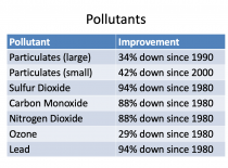
In the post WWII boom, we had problems with air pollution from factories, coal plants, cars, inefficient home heating systems and incinerators in apartments. We had serious air quality issues with pollutants. We had problems with particulates, sulfur dioxide, carbon monoxide, nitrogen oxides, ozone and lead. The worst episodes that really drove efforts to fight pollution were from a atmospheric chemical reactions - cold season water droplets in fog mixed with SO2 to cause sulfuric acid mist. Smog events in Donora PA 1948 led to 6,000 of the 14,000 population to experienced damaged lungs, and the Great London 4 day 1952 Smog Event produced between 10-12,000 deaths.
Events like that still occur in China.

We set standards that had to be met by industry and automakers. After my BS and MS work at Wisconsin in Meteorology, I received a grant to study Air Resources/Pollution at NYU while I worked 7 days a week producing the weather fro WCBS TV and radio and the National Network on the Special series on Energy. Many of my colleagues took jobs dealing with air quality at the EPA and elsewhere, After the work we all did there and at many schools on pollution, we have the cleanest air in my lifetime and here in the U.S. in the world today.
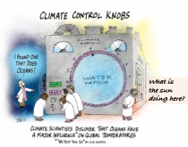
CO2 IS THE GAS OF LIFE
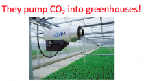
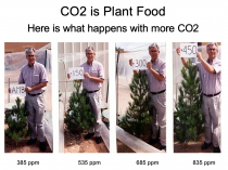
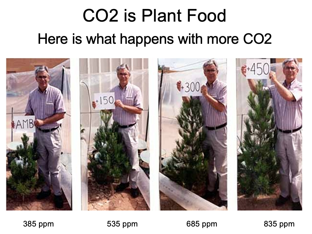
Notice CO2 was not on the list. CO2 is a trace gas (.04% of our atmosphere). It is NOT a pollutant but a beneficial gas. CO2 is essential for photosynthesis. CO2 enriched plants are more vigorous and have lower water needs, are more drought resistant. Ideal CO2 levels for crops would be 3 to 4 times higher. They pump CO2 into greenhouses!
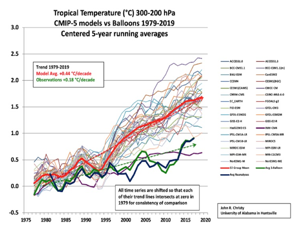
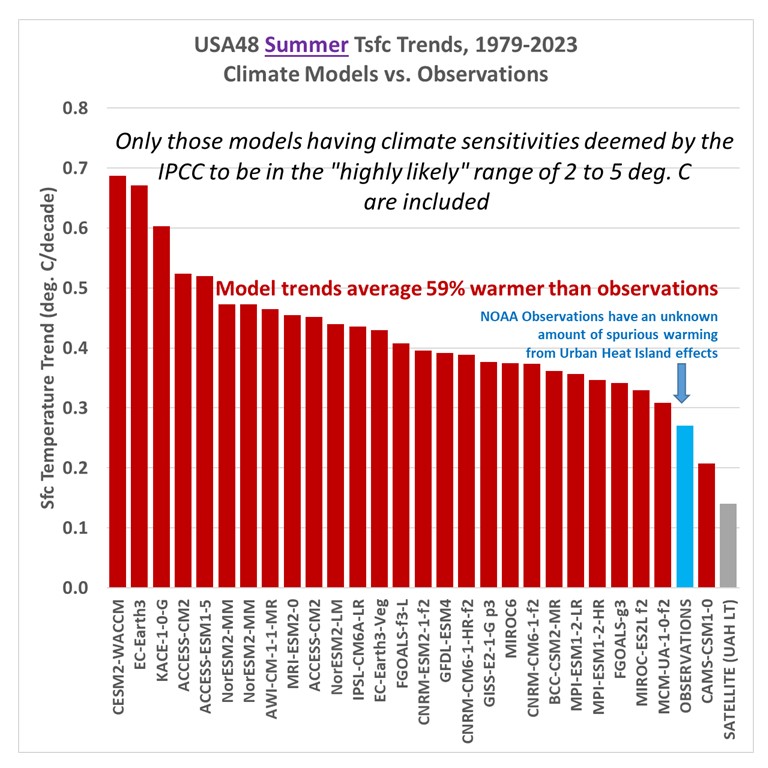
The climate models used to predict the impacts of increasing CO2 deliver warming over 2 times that observed by our NOAA orbiting satellite measurements of the air above the boundary layer where the greatest changes occur diurnally.


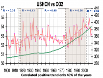
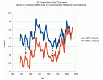
The apparent weak correlation to temperatures may be mostly the timing of the natural cycles. Longer term warming correlates with CO2 increases only 40% of the time.
Enlarged
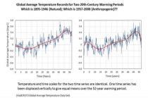
Sadly there have been changes that minimized the warm period from the 1920s to 1940s to try to make the case stronger.
CONCLUSION: CO2 IS NOT POLLUTION BUT A VALUABLE PART OF LIFE ON OUR PLANET
I have 2 CO2 monitors - I bought one - actually using Amazon credits and it arrived the next morning. One high quality model was donated to me to use by the CO2 coalition. I found with my daughter and 2 small dogs in the room, levels rise to over 800. At a football gathering of 8, it rose from 420 to near 1700 ppm. Had our team been doing better, we may have had a gathering with twice a many people and CO2 levels would have been well over 2000. I used and talked about our findings at a church organized meeting.
Many people confuse/conflate CO2 with the potentially deadly CO. That included a decade ago the chair of NH Science and Energy committee when I was one of the testifiers. She said she was taught CO2 was a health hazard (confusing with CO).
I found the story can influence people with open minds. If the CO2 is seen to be locally much higher where people congregate, I am a bit afraid the radical movement and would take that fact on as another cause and try to enforce extreme measures (limiting driving, flying, congregating in large events), to pretend it will keep levels low and it becomes another costly program with much more harm than benefit as their assault on fossil fuel energy usage and the whole COVID episode has been the last 4 years.
-------------
From the CO2 Coalition
According to Patrick Moore, chairman and chief scientist of Ecosense Environmental and co-founder of Greenpeace, the climate change messaging isn’t based in fact.
“The whole thing is a total scam,” said Mr. Moore. “There is actually no scientific evidence that CO2 is responsible for climate change over the eons.”
Mr. Moore said that over the past few decades, the climate message has continually changed; first, it was global cooling, then global warming, then climate change, and now it’s disastrous weather.
This is from Epoch Times and pay walled. Here is a pdf of the article.
------------
I over the years gave many talks on climate - see a recent 50 minute story on local cable.

Here is a much needed compilation from highest level scientists willing to tell the real story. New documentary, “Climate: The Movie” (2024), features Dr. Willie Soon from CERES.
A new documentary on climate change by Martin Durkin, “Climate: The Movie”, was posted online today (March 21st, 2024). The film presents a different perspective on climate change from the standard narratives promoted by the UN’s Intergovernmental Panel on Climate Change (IPCC).
Dr. Willie Soon, CERES co-team leader, was interviewed for this documentary, along with many other scientists and commentators. The 19th century philosopher, John Stuart Mill, noted in 1859 that “he who knows only his own side of the case knows little of that”. This documentary presents a different “side of the case” on climate change, and we think it is definitely worth watching and sharing with anybody who wants to hear different perspectives.
See and share this documentary below.

--------
Three projects I have worked on for the last 2 years have been completed. Together with my regular daily reports on Weatherbell with Joe Bastardi and other superstars, it limited my time on Icecap. I also struggled with the loss of my dear wife Emily, my lifelong companion. I will return to more regular posting and updating the important Alarmist Claim rebuttal work. I appreciate your donations to support the site. SInce our inception, we have had an amazing 271,599,998 views. Thank you!
Steve Goreham in the Washington Examiner,
The next big climate scare is on the way. Advocates of measures to control the climate now propose that we begin counting deaths from climate change. They appear to believe that if people see a daily announcement of climate deaths, they will be more inclined to accept climate change policies. But it’s not even clear that the current gentle rise in global temperatures is causing more people to die.
In December, former Secretary of State Hillary Clinton spoke at COP28, the 28th United Nations Climate Conference, and mentioned climate-related deaths.
“We are seeing and beginning to pay attention and to count and record the deaths that are related to climate,” she said. “And by far the biggest killer is extreme heat.”
---------
See the CO2 coalition video using the actual facts to clearly show the fallacy of this alarmist media and psuedoscientist claims that Steve discusses here:
------------
According to Ms. Clinton, Europe recorded 61,000 deaths from extreme heat in 2023, and she estimated that about 500,000 people died from heat across the world last year.
Global temperatures have been gently rising for the last 300 years. Temperature metrics from NASA, NOAA, and the Climate Research Unit at the University of East Anglia in the United Kingdom estimate that Earth’s surface temperatures have risen a little more than one degree Celsius, or about two degrees Fahrenheit, over the last 140 years. But are these warmer temperatures harmful to people?
According to the Centers for Disease Control and Prevention, most cases of influenza occur during December to March, the cold months in the United States. Influenza season in the southern hemisphere takes place during the cold months there, April through September. The peak months for COVID-19 infections tended to be the cold periods of the year. More people usually get sick during cold months than in warm months.
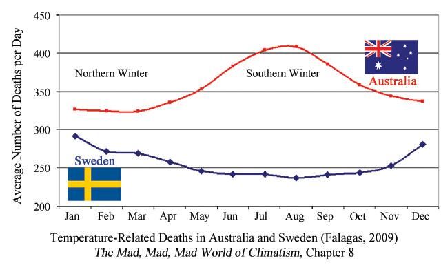
More people also die during winter months than summer months, according to many peer-reviewed studies. For example, Dr. Matthew Falagas of the Alfa Institute of Medical Sciences and five other researchers studied seasonal mortality in 11 nations. The research showed that the average number of deaths peaked in the coldest months of the year in all of them.
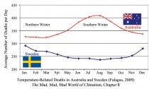
Enlarged: A graph showing the number of countries/regions in the winter
The late Dr. William Keating studied temperature-related deaths in six European countries for people aged 65 to 74. He concluded that deaths related to cold temperatures were nine times greater than those related to hot temperatures. Dr. Bjorn Lomborg, president of the Copenhagen Consensus Center, has pointed out that moderate global warming will likely reduce human mortality.
Yet, on January 30, Dr. Colin J. Carlson of Georgetown University published a paper in Nature Medicine titled, “After millions of preventable deaths, climate change must be treated like a health emergency.” Carlson claims that climate change has caused about 166,000 deaths per year since the year 2000, or almost four million cumulative deaths.
Carlson admits that most of these deaths have been due to malaria in sub-Saharan Africa, or malnutrition and diarrheal diseases in south Asia. But he goes on to claim that deaths due to natural disasters and even cardiovascular disease should also be attributed to climate change. If death from cardiovascular disease can be counted as a climate death, almost any death can be counted.
The evidence doesn’t support these climate death claims. Malarial disease has plagued humanity throughout history, even when temperatures were colder than today. Dr. Paul Reiter, medical entomologist at the Pasteur Institute in Paris, points out that malaria was endemic to England 400 years ago during the colder climate of the Little Ice Age. The Soviet Union experienced an estimated 13 million cases of malaria during the 1920s, with 30,000 cases occurring in Archangel, a city located close to the frozen Arctic Circle.
Malnutrition has been declining during the gentle warming of the last century. During the early 1900s, as many as 10 million people would die from famine each decade globally. Today, world famine deaths have been reduced to under 500,000 people per decade. About 10% of the world’s people are malnourished today, but this is down from about 25% in 1970.
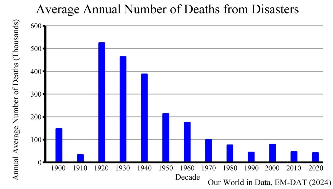
The number of deaths from natural disasters has also been falling during the warming over the last century. According to EM-DAT, the International Disaster Database, the deaths from disasters, including storms, famines, earthquakes, droughts, and floods, are down more than 90 percent over the last 100 years.
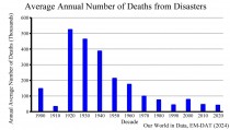
With deaths from natural disasters and famine declining, and since fewer people die in warmer temperatures, the case for counting deaths from global warming is poor at best. But don’t underestimate the ability of climate alarmists to create fear by exaggerating the data.
Steve Goreham is a speaker on energy, the environment, and public policy and the author of the new bestselling book Green Breakdown: The Coming Renewable Energy Failure.
------------------
Icecap Note: Any warming not related to ocean, solar cycles or volcanism is driven by urbanization. NCEI has a data set(s) that are protected from the urban warming contamination by better instrumentation and especially better siting.
In the very first US operational data set in the late 1980s, adjustments were built in to correct for urbanization in the national network in growing cities and 70% of the network stations that were airport. In the following versions the original adjustment algorithms were removed and a data trace that better mapped the AGW claims of man made CO2 warming. Fortunately NOAA with a push from Dr. John Christy, set up a network of carefully sited stations as he used in Alabama where he was the state climatologist. NOAA never discusses this data gem but makes the data available monthly if you can find it on their site. See even with the warming globally that may be driven in part the last few years by TONGA (see) and also on WUWT, the warming trend is minimal.
May 2024 | 1.21F (0.67C)
US Climate Reference Network (data updated 10-15th of month)
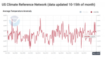
Click for description of the data/larger graph
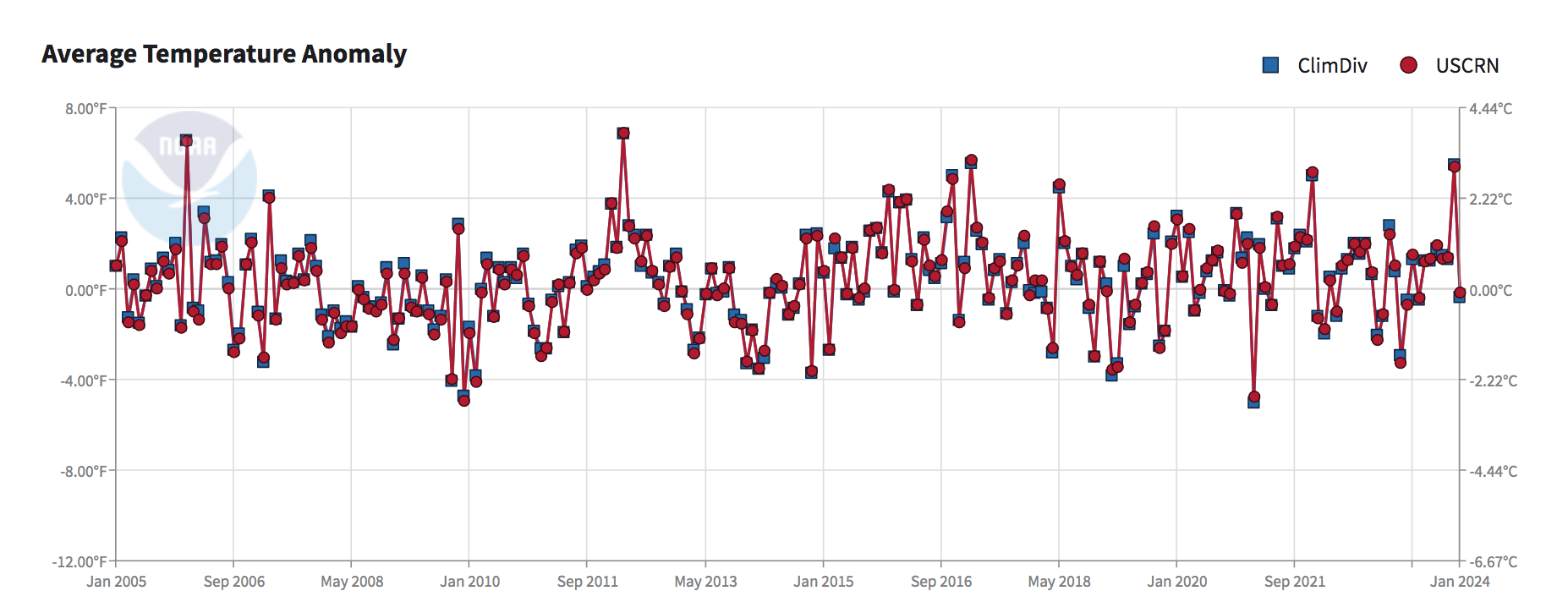
The US Climate Reference Network record from 2005 shows no obvious warming during this period. The graph above is created monthly by NOAA.
The graph shows the Average Surface Temperature Anomaly for the contiguous United States since 2005. The data comes from the U.S. Climate Reference Network (USCRN) which is a properly sited (away from human influences and infrastructure) and state-of-the-art weather network consisting of 114 stations in the USA.
These station locations were chosen to avoid warm biases from Urban Heat Islands (UHI) effects as well as microsite effects as documented in the 2022 report Corrupted Climate Stations: The Official U.S. Surface Temperature Record Remains Fatally Flawed. Unfortunately, NOAA never reports this data in their monthly or yearly “state of the climate report.” And, mainstream media either is entirely unaware of the existence of this data set or has chosen not to report on this U.S. temperature record.
The national USCRN data, updated monthly as shown in the above graph can be viewed here and clicking on ClimDiv to remove that data display in the graph here.
---------
See a history of weather data changes and manipulations over time here.
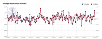
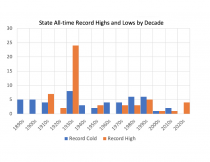
They ignore the actual heat records. The 1930s were clearly the hottest years for all-time state record highs. There have been more record lows than all time highs since then.
Largest Protest in Human History is Under Way in Germany Against the Global Warming Cult
One of the most well-coordinated and massive protests in human history is happening in Europe right now. Blue collar and white collar workers are protesting the EU’s global warming insanity in an ingenious manner that has basically crippled the German economy.
If you haven’t heard anything about this here in America yet, that is because most of our media is on the side of globalist tyranny and against the people. The protests were initially described as another “farmer protest” in Germany, but they have grown into something much larger than that now.
Farms have been under a full-on assault by the global warming cultists and the WEF for a while now. Joe Biden’s “climate envoy” John Kerry has been running around claiming that family farms are going to have to be confiscated from people if we are going to save the planet from the weather. He actually says that. Out loud.
In the EU, that insanity is becoming a reality. The Irish government, for example, passed a law demanding that 1.3 million cows be slaughtered, so that their farts won’t hurt the weather. If the disruption to the global food supply causes lots of people to starve to death, well, that’s a feature of saving the planet from cow farts. You’ve got to break a few eggs in order to make a communist omelet and so forth.
The government has already killed about 10% of the livestock in the Netherlands. That’s a big part of the reason why the “farmer protests” happened in that country. World governments are basically telling “the little guy” that if they lose their livelihood or if they die, that’s a small price to pay for the greater good - for the earth.
Which brings us to the German protests this week.
The German government is trying to impose new restrictions on farms that will basically put small farms out of business. This is exactly the type of policy that John Kerry, who has never been on a farm in his life, is talking about.
Here’s how the amazing German protests have been unfolding.
On day one, the farmers started the protest. They drove their tractors into the cities and started blocking transport hubs, main arteries, and access to government buildings. It’s a nuisance, but the globalists figure they can outlast the farmers while vilifying them and calling them “threats to democracy.”
On day two...a huge number of Polish truck drivers crossed the border into Germany and joined the protest. They blocked even more main highways and shut down the border crossings in and out of Germany. If you’re a globalist in the German government, at this point you’ve got to be thinking, “Uh oh!”
On day three...all the rail workers in Germany went on strike in solidarity with the farmers. Now there are no trains running. The subways are not taking workers to the office. Those trains and trucks loaded with groceries that restock the store shelves in the cities are not coming. And Berlin has about three days’ worth of food on the grocery shelves. Who do you think is going to blink first in this situation?
If the trains aren’t running, then transport companies are forced to use trucks. But the truckers are standing in solidarity with the farmers. The farmers are blocking off the highways and main roads.
How long do you suppose people in Berlin will be willing to go hungry before they step out in solidarity against their fascist, globalist government?
The globalists like to pretend that “the little guy” doesn’t matter. They’re about to learn a painful lesson in Germany. The most important person in your society is not some government bureaucrat with a master’s degree in city administration who works in the Redundant Department of Official Redundancy.
The most important people in society have always been the guys who grow and provide the milk, eggs, cheese, steak, chicken, bread, salads, and bacon (especially bacon) that we all need to survive.
Globalism and neoliberalism have been abject failures. This is why nationalism is the way forward out of the mess that these people have made of the world. It’s why the people are revolting against their governments, by electing nationalist and populist leaders like Javier Milei and Donald Trump.
Tucker Carlson brings us a snapshot of these amazing, multi-dimensional protests in Germany in this short clip: One of the most well-coordinated and massive protests in human history is happening in Europe right now. Blue collar and white collar workers are protesting the EU’s global warming insanity in an ingenious manner that has basically crippled the German economy.
If you haven’t heard anything about this here in America yet, that’s because most of our media is on the side of globalist tyranny and against the people. The protests were initially described as another “farmer protest” in Germany, but they have grown into something much larger than that now.
Farms have been under a full-on assault by the global warming cultists and the WEF for a while now. Joe Biden’s “climate envoy” John Kerry has been running around claiming that family farms are going to have to be confiscated from people if we are going to save the planet from the weather. He actually says that. Out loud.
In the EU, that insanity is becoming a reality. The Irish government, for example, passed a law demanding that 1.3 million cows be slaughtered, so that their farts won’t hurt the weather. If the disruption to the global food supply causes lots of people to starve to death, well, that’s a feature of saving the planet from cow farts. You’ve got to break a few eggs in order to make a communist omelet and so forth.
The government has already killed about 10% of the livestock in the Netherlands. That’s a big part of the reason why the “farmer protests” happened in that country. World governments are basically telling “the little guy” that if they lose their livelihood or if they die, that’s a small price to pay for the greater good-for the earth.
Which brings us to the German protests this week.
The German government is trying to impose new restrictions on farms that will basically put small farms out of business. This is exactly the type of policy that John Kerry, who has never been on a farm in his life, is talking about.
Here’s how the amazing German protests have been unfolding.
On day one, the farmers started the protest. They drove their tractors into the cities and started blocking transport hubs, main arteries, and access to government buildings. It’s a nuisance, but the globalists figure they can outlast the farmers while vilifying them and calling them “threats to democracy.”
On day two...a huge number of Polish truck drivers crossed the border into Germany and joined the protest. They blocked even more main highways and shut down the border crossings in and out of Germany. If you’re a globalist in the German government, at this point you’ve got to be thinking, “Uh oh!”
On day three...all the rail workers in Germany went on strike in solidarity with the farmers. Now there are no trains running. The subways are not taking workers to the office. Those trains and trucks loaded with groceries that restock the store shelves in the cities are not coming. And Berlin has about three days’ worth of food on the grocery shelves. Who do you think is going to blink first in this situation?
If the trains aren’t running, then transport companies are forced to use trucks. But the truckers are standing in solidarity with the farmers. The farmers are blocking off the highways and main roads.
How long do you suppose people in Berlin will be willing to go hungry before they step out in solidarity against their fascist, globalist government?
The globalists like to pretend that “the little guy” doesn’t matter. They’re about to learn a painful lesson in Germany. The most important person in your society is not some government bureaucrat with a master’s degree in city administration who works in the Redundant Department of Official Redundancy.
The most important people in society have always been the guys who grow and provide the milk, eggs, cheese, steak, chicken, bread, salads, and bacon (especially bacon) that we all need to survive.
Globalism and neoliberalism have been abject failures. This is why nationalism is the way forward out of the mess that these people have made of the world. It’s why the people are revolting against their governments, by electing nationalist and populist leaders like Javier Milei and Donald Trump.
Tucker Carlson brings us a snapshot of these amazing, multi-dimensional protests in Germany in this short clip:
See also Public Charging Stations Turn into Electric ‘Car Graveyards’ in Bitter Chicago Cold here
See this by Robert Bryce on “Tesla In Turmoil: The EV Meltdown In 10 Charts” and the Manhattan Contrarian post here on the demise of the US green energy transition.
Weather Rant by Professor Art Horn, Meteorologist AMS
“What is necessary for the very existence of science and what the characteristics of nature are, are not to be determined by pompous preconditions, they are determined always by the material with which we work, by nature herself.” - Dr. Richard Feynman
Published at theartofweather.net
Tuesday September 5th, 2023
Love that quote by the good doctor above. It’s especially relevant to the story below! Be it scientific journals or from the sea of both established and fledgling media companies, they all have one goal it would seem and it’s not the truth but perhaps just part of the truth so that fits their predetermined narrative. Is a lie of omission really a lie or is it a willful desire to deceive (a lie) by appearing to tell the truth?
The story below is also instructive in that it should make one aware of the fact that the big government that is now in power is throwing BILLIONS of dollars at climate scientists and research facilities via the EPA, The National Science Foundation and a myriad of other federal agencies to propel their narrative that climate change is a serious threat to our future.
Follow
Top scientist Patrick Brown says he deliberately OMITTED key fact in climate change piece he’s just had published in prestigious journal to ensure woke editors ran it - that 80% of wildfires are started by humans
Story by Lewis Pennock For Dailymail.Com
A climate change scientist has claimed the world’s leading academic journals reject papers which don’ ‘support certain narratives’ about the issue and instead favor ‘distorted’ research which hypes up dangers rather than solutions.
Patrick T. Brown, a lecturer at Johns Hopkins University and doctor of earth and climate sciences, said editors at Nature and Science - two of the most prestigious scientific journals - select ‘climate papers that support certain preapproved narratives’.
In an article for The Free Press, Brown likened the approach to the way ‘the press focus so intently on climate change as the root cause’ of wildfires, including the recent devastating fires in Hawaii. He pointed out research that said 80 percent of wildfires are ignited by humans.
Brown gave the example of a paper he recently authored titled ‘Climate warming increases extreme daily wildfire growth risk in California’. Brown said the paper, published in Nature last week, ‘focuses exclusively on how climate change has affected extreme wildfire behavior’ and ignored other key factors.
Brown laid out his claims in an article titled ‘I Left Out the Full Truth to Get My Climate Change Paper Published’. ‘I just got published in Nature because I stuck to a narrative I knew the editors would like. That’s not the way science should work,’ the article begins.
‘I knew not to try to quantify key aspects other than climate change in my research because it would dilute the story that prestigious journals like Nature and its rival, Science, want to tell,’ he wrote of his recently-published work.
‘This matters because it is critically important for scientists to be published in high-profile journals; in many ways, they are the gatekeepers for career success in academia. And the editors of these journals have made it abundantly clear, both by what they publish and what they reject, that they want climate papers that support certain preapproved narratives - even when those narratives come at the expense of broader knowledge for society.
“To put it bluntly, climate science has become less about understanding the complexities of the world and more about serving as a kind of Cassandra, urgently warning the public about the dangers of climate change. However understandable this instinct may be, it distorts a great deal of climate science research, misinforms the public, and most importantly, makes practical solutions more difficult to achieve.’
A spokesperson for Nature said ‘all submitted manuscripts are considered independently on the basis of the quality and timeliness of their science’.
‘Our editors make decisions based solely on whether research meets our criteria for publication - original scientific research (where conclusions are sufficiently supported by the available evidence), of outstanding scientific importance, which reaches a conclusion of interest to a multidisciplinary readership,’ a statement said.
‘Intentional omission of facts and results that are relevant to the main conclusions of a paper is not considered best practice with regards to accepted research integrity principles,’ the spokesperson added.
Science was approached for comment.
Brown opened his missive with links to stories by AP, PBS NewsHour, The New York Times and Bloomberg which he said give the impression global wildfires are ‘mostly the result of climate change’.
He said that ‘climate change is an important factor’ but ‘isn’t close to the only factor that deserves our sole focus’.
Much reporting of the wildfires in Maui has said climate change contributed to the disaster by helping to create conditions that caused the fires to spark and spread quickly.
The blazes, which killed at least 115 people, are believed to have been started by a downed electricity line, but observers have said rising temperatures caused extremely dry conditions on the Hawaiian island.
Brown said the media operates like scientific journals in that the focus on climate change ‘fits a simple storyline that rewards the person telling it’.
Scientists whose careers depend on their work being published in major journals also ‘tailor’ their work to ‘support the mainstream narrative’, he said.
‘This leads to a second unspoken rule in writing a successful climate paper,’ he added. ‘The authors should ignore - or at least downplay - practical actions that can counter the impact of climate change.’
He gave examples of factors which are ignored, including a ‘decline in deaths from weather and climate disasters over the last century’. In the case of wildfires, Brown says ‘current research indicates that these changes in forest management practices could completely negate the detrimental impacts of climate change on wildfires’.
Poor forest management has also been blamed for a record number of wildfires in Canada this year.
But ‘the more practical kind of analysis is discouraged’ because it ‘weakens the case for greenhouse gas emissions reductions’, Brown said.
Successful papers also often use ‘less intuitive metrics’ to measure the impacts of climate change because they ‘generate the most eye-popping numbers’, he said.
He went onto to claim that other papers he’s written which don’t match a certain narrative have been ‘rejected out of hand by the editors of distinguished journals, and I had to settle for less prestigious outlets’.
Brown concluded: ‘We need a culture change across academia and elite media that allows for a much broader conversation on societal resilience to climate. The media, for instance, should stop accepting these papers at face value and do some digging on what’s been left out.’
‘The editors of the prominent journals need to expand beyond a narrow focus that pushes the reduction of greenhouse gas emissions. And the researchers themselves need to start standing up to editors, or find other places to publish.’
ICECAP NOTE: See a telling media story on the deadly Maui wildfires real causes here and more here.
------------
By Francis Menton,
We highly recommend this site for science and data based related stories on climate and energy policies in this world where “stupidity rules”.
On May 23, EPA put out its long-expected proposed Rule designed to eliminate, or nearly so, all so-called “greenhouse gas” emissions from the electricity-generation sector of the economy. The proposal came with the very long title: “New Source Performance Standards for GHG Emissions from New and Reconstructed EGUs; Emission Guidelines for GHG Emissions from Existing EGUs; and Repeal of the Affordable Clean Energy Rule.” The full document is 672 pages long.
Various not-very-far-off deadlines are set, ranging from as early as 2030 for some changes to coal plants, to at the latest 2038 for the last changes to natural gas plants. But how exactly is this emissions elimination thing to be accomplished? Today a substantial majority of U.S. electricity (about 60%) comes from one or the other of those fuels; and it is inherent in the burning of hydrocarbons that you get CO2 as a product. In all those 672 pages, EPA has only two ideas for how to eliminate the carbon emissions from combustion power plants: carbon capture and storage (CCS), and “green” hydrogen. Either you must implement one of those two ideas to meet EPA’s standards by the deadline, or you must close your power plant. But here’s the problem: both of those ideas are, frankly, absurd.
The deadline for commenting on the proposed Rule was August 8, although comments have continued to pile in after that date. Many hundreds of them have been received. If you have nothing else to do for the next month or two, you can review the comments at this link.
I have by no means made the effort to read all the comments, but I have gone looking for some of the more significant ones. Two that I can highly recommend are this one by a group of 21 red state AGs led by West Virginia, and this one by an overlapping group of 18 red state AGs led by Ohio. Both of those comments do an excellent job of dismantling the concept that either CCS or “green” hydrogen could ever work as a significant part of our electricity generation system. Of the two, the West Virginia comment is the much longer (54 pages) and goes into far more technical detail. But the Ohio comment, at 21 pages, has its share of good zingers as well.
The Ohio and West Virginia comments label the idea of CCS at the high rate demanded by EPA (90%) as either “infeasible” or not “viable,” and include recitations of the history of failed attempts to implement this frankly useless technology. From the Ohio comment (page 4):
A study of 263 carbon-capture-and-sequestration projects undertaken between 1995 and 2018 found that the majority failed and 78% of the largest projects were cancelled or put on hold. After the study was published in May 2021, the only other coal plant with a carbon-capture-and-sequestration attachment in the world, Petra Nova, shuttered after facing 367 outages in its three years of operation.
With the closure of Petra Nova, there remains in the entire world exactly one operating commercial CCS facility at a coal power station, the SaskPower Boundary Dam Unit 3 in Saskatchewan, Canada. That one is supposed to achieve the 90% capture rate that EPA demands, but with constant operating issues it has fallen way, way short:
[T]his [SaskPower] facility is the world’s only operating commercial carbon capture facility at a coal-fired power plant. And it has never achieved its maximum capacity. It also battled significant technical issues throughout 2021- to the point that the plant idled the equipment for weeks at a time. As a result, the plant achieved less than 37% carbon capture that year despite having an official target of 90%…
The West Virginia comment provides lots more technical detail on the failures of CCS. Why can’t a CCS system just easily suck up all the CO2 out of a power plant’s emissions stream? Because the effort to suck up the emissions takes energy from the output of the plant, and the higher the percentage of carbon emissions you seek to capture, the more of the energy output of the plant you consume. (I have previously described CCS efforts as a “war against the second law of thermodynamics."). In the limiting case, you can use up all the power output of the plant on the CCS system and still not capture 100% of the CO2. From the West Virginia comment, page 24-25:
Take efficiency to start. CCS units run on power, too. An owner can get that power from the plant itself. But this approach makes the plant less efficient by increasing its “parasitic load"-and CCS more than triples combustion turbines’ normal parasitic load… This is the cause the Wyoming study analyzed that showed installing CCS technology would devastate plants’ heat rates and lower net plant efficiency by 36%.
And that percentage relates to a system that captures well less than 100% of the plant’s carbon emissions. And these are only the start of the technical issues to be faced. For example, once you have captured all this CO2, where do you put it? Do you build an entire new national network of pipelines (at a cost of hundreds of billions of dollars) to transport it to some underground caverns somewhere? And then, are there environmental issues with the chemicals used to snag the CO2 out of the power plant’s emissions stream? From the West Virginia comment, page 27:
The Proposed Rule would force utilities to adopt and communities to accept all aspects of CCS technology without fully understanding the ramifications. For example, the environmental and health effects of CANSOLV-the leading amine-based and EPA-recommended CCS solvent, 88 Fed. Reg. at 33,291- appear unknown; leading CANSOLV studies over the past decade don’t discuss its impact.
And then, if you have to increase the power output of the plant by 50% or so to power the CCS facility, doesn’t that then increase the emissions of nitrous oxides and particulates by a comparable amount? From the West Virginia comment, page 27:
Nearly a decade ago, the European Union’s European Environmental Agency released a study finding that CCS would increase “direct emissions of NOx and PM” by nearly a half and a third, respectively, because of additional fuel burned, and increase “direct NH3 emissions” “significantly” because of “the assumed degradation of the amine-based solvent.”
It goes on and on from there. And then there’s the idea of “co-firing” the power plants with “green” hydrogen, produced by using wind or solar power or something else magical to electrolyze water. EPA’s proposed Rule would impose such a requirement on existing natural gas plants to take them up to 96% hydrogen by 2038. A few insights from the West Virginia comment, page 35:
Most combustion turbines on the market today cannot handle anything more than a 5-10% blend [of hydrogen]; 20% is generally accepted as the absolute technological ceiling… Even in the best scenarios, a hydrogen volume fraction of 20% is usually the most technology currently can do.
And how about the problem (and cost) of producing the amounts of hydrogen that would be required. From the West Virginia comment, page 37:
America currently produces just .5% of the clean hydrogen we need under the Proposed Rule. The industry would have to close a 99.5% supply gap in just 15 years. EPA has offered no evidence showing that this gap will close.
There is much, much more on issues like transporting and handling the hydrogen, cost of production, and so forth.
The conclusion is obvious and impossible to escape: These proposed methods to allow combustion power plants to continue to exist are not real and can never work. EPA intends to force the closure of all such electricity generation facilities. Will we have an electricity system that can still function at that point? They neither know nor care. After all, we have a planet to save here.
Somehow, in the weighing of the costs and benefits here, the bureaucrats appear to have completely lost track of the enormous benefits that reliable access to electricity has brought to the people. They will destroy that without giving the subject a second thought.
By Steve Goreham
Originally published in The Western Journal.

Which is more environmentally friendly, an energy source that uses one unit of land to produce one unit of electricity, or a source that uses 100 units of land to produce one unit of electricity? The answer should be obvious. Nevertheless, green energy advocates call for a huge expansion of wind, solar, and other renewables that use vast amounts of land to replace traditional power plants that use comparatively small amounts of land.
Vaclav Smil, professor emeritus of the University of Manitoba in Canada, extensively analyzed the power density of alternative sources used to generate electricity. He defined the power density of an electrical power source as the average flow of electricity generated per square meter of horizontal surface (land or sea area). The area measurement to estimate power density is complex. Smil included plant area, storage yards, mining sites, agricultural fields, pipelines and transportation, and other associated land and sea areas in his analysis.
Smil’s work allows us to compare the energy density of electricity sources. If we set the output of a nuclear plant to one unit of land required for one unit of electricity output, then a natural gas-powered plant requires about 0.8 units of land to produce the same one unit of output. A coal-fired plant uses about 1.4 units of land to deliver an average output of one unit of power.
But renewable sources require vastly more land. A stand-alone solar facility requires about 100 units of land to deliver the same average electricity output of a nuclear plant that uses one unit of land. A wind facility uses about 35 units of land if only the concrete wind tower pads and the service roads are counted, but over 800 units of land for the entire area spanned by a typical wind installation. Production of electricity from biomass suffers the poorest energy density, requiring over 1,500 units of land to output one unit of electricity.
As a practical example, compare the Ivanpah Solar Electric Generating System in the eastern California desert to the Diablo Canyon Nuclear Plant near Avila Beach, California. The Ivanpah facility produces an average of about 793 gigawatt-hours per year and covers an area of 3,500 acres. The Diablo Canyon facility generates about 16,165 gigawatt-hours per year on a surface area of 750 acres. The nuclear plant delivers more than 20 times the average output on about one-fifth of the land, or 100 times the power density of the solar facility.
To approach 100 percent renewable electricity using primarily wind and solar systems, the land requirements are gigantic. “Net-Zero America,” a 2020 study published by Princeton University, calls for wind and solar to supply 50 percent of US electricity by 2050, up from about 14 percent today. The study estimated that this expansion would require about 228,000 square miles of new land (590,000 square kilometers), not including the additional area needed for transmission lines. This is an area larger than the combined area of Illinois, Indiana, Iowa, Kentucky, West Virginia, and Wisconsin. This area would be more than 100 times as large as the physical footprint of the coal and natural gas power systems that would be replaced.

The land taken for wind and solar can seriously impact the environment. Stand-alone solar systems blanket fields and deserts, blocking sunlight and radically changing the ecosystem, and driving out plants and animals. Since 2000, almost 16 million trees have been cut down in Scotland to make way for wind turbines, a total of more than 1,700 trees felled per day. This environmental devastation will increase the longer Net Zero goals are pursued.
Wind and solar are dilute energy. They require vast amounts of land to generate the electricity required by modern society. Without fears about human-caused global warming, wind and solar systems would be considered environmentally damaging. Net-zero plans for 2050, powered by wind and solar, will encounter obstacles with transmission, zoning, local opposition, and just plain space that are probably impossible to overcome.
Steve Goreham is a speaker on energy, the environment, and public policy and the author of the new book Green Breakdown: The Coming Renewable Energy Failure.
by Ron Barmby
Political tunnel vision on global warming has resulted in declaring increases in atmospheric carbon dioxide an existential threat. But the United Nations’ resolve to reduce carbon dioxide levels runs counter to its goals to end world hunger, promote world peace and protect global ecosystems. It fails to address the key question relating to those three goals: Which pathway creates the greatest good to the greatest multitude - reducing or increasing CO2?
The numbers since the year 2000 provide convincing evidence that increasing carbon dioxide has positive impacts and reducing carbon emissions entails dire consequences.
World Hunger
The pre-industrial (circa 1850) atmospheric CO2 concentration of 280 ppm (parts per million) compares to today’s 420 ppm, a 50% increase. Meanwhile, the global population has risen 560%, from 1.2 billion to 8 billion.
Those extra 6.8 billion people are mostly being fed, and it’s not all because of human agricultural productivity, pest control and plant genetics.
Observations of Earth’s vegetative cover since the year 2000 by NASA’s Terra satellite show a 10% increase in vegetation in the first 20 years of the century. Clearly, something other than agriculture is helping to improve overall plant growth.
In a recent study supported by the U.S. Department of Energy, Dr. Charles Taylor and Dr. Wolfram Schlenker quantified how much of that extra greening resulted in food for human consumption since 2000. Using satellite imagery of U.S. cropland, they estimated that a 1 ppm increase in CO2 led to an increase of 0.4%, 0.6% and 1% in yield for corn, soybeans and wheat, respectively. They also extrapolated back to 1940 and suggested that the 500% increased yield of corn and 200% increased yield of soybeans and winter wheat are largely attributable to the 100 ppm increase in CO2 since then.
CO2 fertilization is not only greening the Earth, it’s feeding the very fertile human race.
World Peace
Though adding CO2 to the atmosphere does not promote world peace, attempts to stop CO2 emissions in the western democracies have increased the CO2 emissions, wealth and influence of totalitarian Russia and China.
Eurostat, the statistical office of the European Union (EU), reports that the EU’s reliance on imported natural gas increased from 15.5% of its energy needs in 2000 to 22.5% by 2020. Russia was the main supplier of Europe’s natural gas. Holding Europe’s energy security in its pipelines not only helped finance Russia’s 2021 invasion of Ukraine, but it also limited the economic sanctions Europe could impose in retaliation.
According to the scientific online publication Our World in Data, between 2000 and 2020 the G7 nations lost 13.8% of the world share of GDP and China picked up 12%.
The West (the EU plus the UK, U.S., Canada and Japan) transferred GDP growth to China and energy security to Russia and was able to reduce CO2 emissions from 45% of the global total in 2000 to 25% in 2020. In the same period China’s CO2 emissions grew from 14% of the total to 31%, leading to an increase of 39% in total CO2 global emissions.
The unintended consequence of the West’s attempts to reduce CO2 emissions has been to shore up Chinese and Russian dictatorships-and in Russia’s case, to partly fund the invasion of a sovereign and democratic neighbor, Ukraine.
World Ecology
Much of the human footprint on Earth is where the products we consume originate: We either grow them on the planet’s surface or extract them from within its crust.
In testimony to the U.S. House Committee on Energy and Commerce in 2021, Mark Mills, a senior fellow at the Manhattan Institute, estimated that replacing each unit of hydrocarbon energy by “clean tech” energy would on average result in the extraction of five to 10 times more materials from the Earth than does hydrocarbon production.
Mills also pointed out that Chinese firms dominate the production and processing of many critical rare earth elements and that nearly all the growth in mining is expected to be abroad, increasingly in fragile, biodiverse wilderness areas.
Decarbonization will impose the heavy environmental cost of an unprecedented increase in mining.
One Last Number
Since El Nino induced a modern peak global average temperature in 1998, global warming has been essentially zero.
The numbers don’t lie. Allowing more CO2 emissions is better for ending world hunger, promoting world peace, and protecting global ecosystems.
This commentary was first published at Real Clear Energy, July 6, 2023, and can be accessed here.
Ron Barmby, a Professional Engineer with a master’s degree in geosciences, had a 40-year career in the energy industry that covered 40 countries and five continents. He is author of “Sunlight on Climate Change: A Heretic’s Guide to Global Climate Hysteria” and is a proud member of the CO2 Coalition, Arlington, Virginia.
Scientific Paper Concludes Refrigerants’ Gases Pose No Threat to Climate
CO2 Coalition, 28 June
The paper examines the warming potential of 14 halogenated gases, which are more specifically identified as hydrochlorofluorocarbons (HCFCs) and hydrofluorocarbons (HFCs). The gases are to be phased out as refrigerants because of their purported threat of dangerously warming the climate. The ban on these chemicals is being imposed under amendments to a 1987 international agreement known as the Montreal Protocol, which forced the abandonment of freon as a refrigerant because of concerns about that chemical’s capacity to destroy ozone in the upper atmosphere. The U.S. Senate ratified the so-called Kilgali amendment to the Montreal Protocol in 2022. Drs. Van Wijngaarden and Happer conclude that the 14 gases’ contribution to atmospheric warming amounts to only 0.002 degrees C per decade, a warming indistinguishable from zero.
-----------
School Official Laments Cost and Performance of Electric Buses
Heather Hamilton, Washington Examiner, 29 May
One Michigan school official admitted his district’s move to using electric was less than the government has touted it to be. “Electric buses are approximately five times more expensive than regular buses, and the electrical infrastructure, which was originally estimated to be only about $50,000, give or take, for those four buses ended up being more like $200,000.
------------
Wind Fails Texas Again
Bill Peacock, Master Resource, 26 June
Wind’s market share is far higher in temperate months than in the hot summer months or the cold winter months when loads are heavy and generation is needed. In March, April, May, October, and November, wind’s market share is 31.7%. In the winter months of December, January, and February, wind’s market share drops to 25.7%. In the summer months of June, July, August, and September, wind’s market share plummets to 18.1%.
-----------
Baseball Sized Hail Smashing into Panels at 150 MPH Destroys Scottsbluff Solar Farm
Kevin Killough, Cowboy State Daily, 27 June
Baseball-sized hail took out a solar farm in Scottsbluff, Nebraska, on Friday. The hail shattered most of the panels on the 5.2-megawatt solar project, sparing an odd panel like missing teeth in a white smile. “Just by looking at it, it looks destroyed to me,” [Scottsbluff city manager Kevin] Spencer said.
-----------
London ULEZ Expansion Will Force 40% of Drivers To Give Up Their Cars in August
Felix Reeves, Express, 23 June
A new study has found that two in five Londoners will be forced to change or give up their current car under the expansion of the Ultra Low Emission Zone coming into force in just over two months.
-----------
EU Looks Into Blocking Out the Sun as Climate Efforts Falter
John Ainger, Bloomberg Green, 26 June
The European Union will join an international effort to assess whether large-scale interventions such as deflecting the sun’s rays or changing the Earth’s weather patterns are viable options for fighting climate change.
By Meteorologist Art Horn
“The opinions that are held with passion are always those for which no good ground exists; indeed the passion is the measure of the holders lack of rational conviction.”
-Bertrand Russell 10/10/21
Published at theartofweather.net
Wednesday June 7th, 2023
There’s just too much going on not to talk about it. To quote Jack Klompus from Seinfeld “I’m sorry. I’m sitting here, the whole meeting, holding my tongue. I’ve known you a long time Morty, but I cannot hold it in any longer.”
I’m referring to the current situation of the Canadian wildfires and the resulting and persistent smoke issues down here in the United States. Under normal conditions a large very slow-moving storm rotating counterclockwise in the Canadian Maritimes would be circulating cool, dry, clean Canadian air into the New England. There is such a storm present in that location now. But with all these fires in Quebec Province the storm that is situated in the Maritimes is doing the opposite! The smoke from the fir...ta. In court on February 15th, 2022 she was convicted on four counts of mischief against property in connection with multiple arson fires in the Bonnyville area of Alberta Canada. She actually admitted to setting 32 fires at the hearing! Apparently she was quite proud of her destruction. She was sentenced to 9 months in jail but amazingly she served no jail time.
Can I prove that at least some of these current fires have been deliberately set by eco-terrorists? No, not until someone claims responsibility or is arrested but it seems plausible to me.
Why would someone want to destroy forests that they claim they are trying to save? At least part of the answer is that by starting the fires and then blaming the cause on climate change they get the news coverage they couldn’t get any other way. The news media actually does the work for them since they are obsessed with climate change causing everything! Today every natural disaster they report about is now the result of climate change.
As a side note I saw yet another of the seemingly endless stories about sea ice loss in the Arctic. This story from the thedailybeast.com reports that another computer model study forecasts that after the year 2030 there will be no sea ice in the Arctic Ocean by the end of the summer.
Of course, one has to only go back to 2007 when there were similar predictions warning that by 2022 summer sea ice would be long gone from the Arctic. Another in the long line of climate change forecasts fails. Actually, sea ice data from the Danish Meteorological Institute reveals that as of today the amount of Arctic sea ice is within 75 percent of the 1981 to 2010 average for this time of year. Where are you going to see that in the news? Nowhere!
-----------
Note: Mark Perry on Carpe Diem here listed 18 major failures.
“Most of the people who are going to die in the greatest cataclysm in the history of man have already been born,” wrote Paul Ehrlich in a 1969 essay titled “Eco-Catastrophe! “By....[1975] some experts feel that food shortages will have escalated the present level of world hunger and starvation into famines of unbelievable proportions. Other experts, more optimistic, think the ultimate food-population collision will not occur until the decade of the 1980s.”
Erlich sketched out his most alarmist scenario for the 1970 Earth Day issue of The Progressive, assuring readers that between 1980 and 1989, some 4 billion people, including 65 million Americans, would perish in the “Great Die-Off.” “It is already too late to avoid mass starvation,” declared Denis Hayes, the chief organizer for Earth Day, in the Spring 1970 issue of The Living Wilderness.
Leonard Nimoy talked about the coming ice age in 1979 here.
Tony Heller exposes the fraudsters here.
Unlike the government, businesses must respect reality or they will go bankrupt.
The reality is that atmospheric CO2 is remarkably beneficial. Exxon knows that the byproducts of burning fossil fuels, carbon dioxide and water, are more than completely benign. They are essential. All life on this planet comes from carbon dioxide and water. If we combine those two ingredients, we get soda water. But if we give them to a plant in the presence of sunlight, it will produce glucose and from that other sugars, starches, fats, proteins, and cellulose. In other words, all life.
What about warming from the Greenhouse Effect? CO2 is a greenhouse gas like water vapor. But water vapor completely dominates that effect, so much that climate alarmists quietly assume that it will produce most of the warming from rising CO2 in the atmosphere. But water vapor is self limiting, such that it does not produce catastrophic warming.
One important way that water vapor controls warming is through the formation of clouds that reflect sunlight back to space, before they can heat the ground.
The most recent winner of the Nobel Prize in Physics, John Clauser, thinks that clouds are the key to understanding our climate, not carbon dioxide. I agree with him and would add the entire hydrological cycle to the negative feedbacks that keep our climate stable.
John Clauser has joined us as a Director of the CO2 Coalition to refute the vast nonsense coming from the scientifically illiterate.
Exxon should be commended for finally standing up to the climate idiots, just like John Clauser is doing.
--------------
Exxon Says World Hitting Mythical “Net-Zero” by 2050 is Nonsense
May 19, 2023
Finally, at least one Big Oil company is willing to go on the record countering the mass insanity of the left. The left wants humanity to kill itself in order to achieve mythical “net zero” (no extra carbon emissions) by 2050. Leftist lunatics have tried to brainwash the world that if we don’t hit net zero (which is impossible), that’s it. Lights out. The world toasts, and we burn ourselves to a cinder. There is no hope for the future. Which is complete nonsense. Exxon said as much in an official statement to shareholders in an SEC filing.
Proxy adviser Glass Lewis told Exxon (and shareholders) the company should prepare for the end of the world-as in the use of fossil fuels will be completely phased out by 2050, leaving Exxon without a business if it doesn’t change its product lines. After picking themselves up off the floor from laughing so hard, Exxon told Glass Lewis, via a response in an SEC filing (below), they are (our words) smoking something funny.
“Glass Lewis apparently believes the likelihood of the IEA NZE scenario is well beyond what the IEA itself contends: that the world is not on the NZE path and that this is a very aggressive scenario,” Exxon said. “It is highly unlikely that society would accept the degradation in global standard of living required to permanently achieve a scenario like the IEA NZE.”
In other words, ain’t no way people are ready to go back to the Stone Age and never travel beyond five miles from their homes. Ain’t no way people will give up their iPhones. Ain’t no way folks will throw on an extra sweater or two or three in the winter to keep warm. There ain’t no way to actually manufacture cars light enough to run on batteries-without fossil fuels to make the plastic! It’s bizarre. And yet, that’s what the weenies at Glass Lewis say is going to happen.
Exxon Mobil Corp. said the prospect of the world reaching net zero carbon dioxide emissions by 2050 is “highly unlikely” due to the drop in living standards that would come with such a scenario.
The Texas oil giant made the comments in a regulatory filing that argued against proxy adviser Glass Lewis’ view that the cost of phasing out oil and gas operations would be a material financial risk. The International Energy Agency’s Net Zero Emissions scenario, which models a phaseout of most fossil fuels by 2050, has little bearing in reality, Exxon said.
“Glass Lewis apparently believes the likelihood of the IEA NZE scenario is well beyond what the IEA itself contends: that the world is not on the NZE path and that this is a very aggressive scenario,” Exxon said. “It is highly unlikely that society would accept the degradation in global standard of living required to permanently achieve a scenario like the IEA NZE.”
Climate pledges by governments would fall short of net zero by 2050 even if they were achieved, meaning there’s little chance of limiting global temperature increases to 1.5 degrees Celsius above preindustrial levels, according to the IEA. Exxon has a net zero “ambition” by 2050 but is investing heavily in new projects - both fossil fuels and low carbon - that it believes will provide the flexibility to respond to multiple energy transition scenarios.
Exxon urged shareholders to reject a resolution, backed by Glass Lewis, that the company should produce a report at its annual meeting on May 31 on the cost of shutting oil and gas operations that no longer are needed.
ICECAP NOTE:
In addition to reporting the recent warm period is less than half that predicted by the greenhouse models, Happer and Lindzen showed the recent 50 year period 1957-2008 was a match to the 1895 to 1946 cooling then warming which the so-called scientists at the IPCC ignore or admit that was natural.
By Ross McKitrick is a professor of economics at the University of Guelph and senior fellow of the Fraser Institute.
An important new study on climate change came out recently. I’m not talking about the Intergovernmental Panel on Climate Change (IPCC) Synthesis Report with its nonsensical headline “Urgent climate action can secure a liveable future for all.” No, that’s just meaningless sloganeering proving yet again how far the IPCC has departed from its original mission of providing objective scientific assessments.
I’m referring instead to a new paper in the Journal of Geophysical Research-Atmospheres by a group of scientists at the U.S. National Oceanic and Atmospheric Administration (NOAA) headed by Cheng-Zhi Zou, which presents a new satellite-derived temperature record for the global troposphere (the atmospheric layer from one kilometre up to about 10 km altitude).
The troposphere climate record has been heavily debated for two reasons. First, it’s where climate models say the effect of warming due to greenhouse gases (GHGs) will be the strongest, especially in the mid-troposphere. And since that layer is not affected by urbanization or other changes to the land surface it’s a good place to observe a clean signal of the effect of GHGs.
Since the 1990s the records from both weather satellites and weather balloons have shown that climate models predict too much warming. In a 2020 paper, John Christy of the University of Alabama-Huntsville (UAH) and I examined the outputs of the 38 newest climate models and compared their global tropospheric warming rates over 1979 to 2014 against observations from satellites and weather balloons. All 38 exhibited too much warming, and in most cases the differences were statistically significant. We argued that this points to a structural error in climate models where they respond too strongly to GHGs.
But, and this is the second point of controversy, there have also been challenges to the observational record. Christy and his co-author, Roy Spencer, invented the original method of deriving temperatures from microwave radiation measurements collected by NOAA satellites in orbit since 1979. Their achievement earned them numerous accolades, but also attracted controversy because their satellite record didn’t show any warming. About 20 years ago scientists at Remote Sensing Systems in California found a small error in their algorithm that, once corrected, did yield a warming trend.
Christy and Spencer incorporated the RSS correction, but the two teams subsequently differed on other questions, such as how to correct for the positional drift of the satellites, which changes the time of day when instruments take their readings over each location. The RSS team used a climate model to develop the correction while the UAH team used an empirical method, leading to slightly different results. Another question was how to merge records when one satellite is taken out of service and replaced by another. Incorrect splicing can introduce spurious warming or cooling.
In the end the two series were similar but RSS has consistently exhibited more warming than UAH. Then a little more than a decade ago, the group at NOAA headed by Zou produced a new data product called STAR (Satellite Applications and Research). They used the same underlying microwave retrievals but produced a temperature record showing much more warming than either UAH or RSS, as well as all the weather balloon records. It came close to validating the climate models, although in my paper with Christy we included the STAR data in the satellite average and the models still ran too hot. Nonetheless it was possible to point to the coolest of the models and compare them to the STAR data and find a match, which was a lifeline for those arguing that climate models are within the uncertainty range of the data.
Until now. In their new paper Zou and his co-authors rebuilt the STAR series based on a new empirical method for removing time-of-day observation drift and a more stable method of merging satellite records. Now STAR agrees with the UAH series very closely - in fact it has a slightly smaller warming trend. The old STAR series had a mid-troposphere warming trend of 0.16 degrees Celsius per decade, but it’s now 0.09 degrees per decade, compared to 0.1 in UAH and 0.14 in RSS. For the troposphere as a whole they estimate a warming trend of 0.14 C/decade.
Zou’s team notes that their findings “have strong implications for trends in climate model simulations and other observations” because the atmosphere has warmed at half the average rate predicted by climate models over the same period. They also note that their findings are “consistent with conclusions in McKitrick and Christy (2020),” namely that climate models have a pervasive global warming bias. In other research, Christy and mathematician Richard McNider have shown that the satellite warming rate implies the climate system can only be half as sensitive to GHGs as the average model used by the IPCC for projecting future warming.
Strong implications, indeed, but you won’t learn about it from the IPCC. That group regularly puts on a charade of pretending to review the science before issuing press releases that sound like Greta’s Twitter feed. In the real world the evidence against the alarmist predictions from overheated climate models is becoming unequivocal. One day, even the IPCC might find out.
Ross McKitrick is a professor of economics at the University of Guelph and senior fellow of the Fraser Institute.
The IPCC, the media and the clueless or green evangelists like AOC and are dead wrong and our future well being requires us to expose why. For one, C02 is a minor gas and one that feeds the world. We breath out with every breath 100 times more CO2 that we breathe in. Listen to Dr. Patrick Moore, co-founder of Greenpeace here.
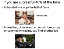
Next let’s look at the success rate of of the climate forecasters.
----------------
Then the very latest global data:
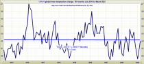
Newly released weather data shows average climates worldwide have remained unchanged for about nine years.
The data published by the National Space Science and Technology Center shows that there has been zero global warming since July of 2015, eight years and nine months ago.
The finding undermines arguments by the Biden administration and others that rising temperatures, in large part the result of emission from fossil-burning fuels, have become an existential threat and that needs to be stopped.
Steve Milloy, a former EPA transition team member for administration and founder of Junkscience.com, tweeted in response to the new data: “Just in… no global warming in 8 years and 9 months...despite 500 billion tons of emissions worth 14% of total manmade CO2. Emissions-driven warming is a hoax.”
--------------
You have a fever with jaundice, feel crappy, and are vomiting.
You go to the emergency room at the local hospital.
The ER doctor does not run any tests, but based on the symptoms his diagnosis is acute alcoholism and prescribes abstinence or you will drink yourself to death.
“What about some tests, or a second opinion?” you ask. The doctor informs you that “the administration in this hospital has two rules: firstly, the only diagnosis we give out for these symptoms is chronic alcohol abuse; and secondly, we delete any data to the contrary from your file.”
You check into rehab but the fever, jaundice, and nausea persist. Six days later you die from acute fulminant viral hepatitis (Hep B). But sober.
A reasonable person would not accept a diagnosis dictated by the hospital administration and the deletion of conflicting data. Especially if you knew acute alcoholic hepatitis and acute viral HBV hepatitis present the same symptoms and it takes blood tests to differentiate them with certainty.
And that’s why you should ignore the latest Intergovernmental Panel on Climate Change (IPCC) report because two similar rules govern their analysis and reporting. The cure is also similar: Net Zero CO2 by 2050.
The IPCC Report Cycle
The IPCC’s 1988 mandate from the United Nations was to review, “The state of the knowledge of the science of climate and climatic change”.
In that mandate, the UN expressed “concern that human activities could change global climate patterns, threatening present and future generations...” and also includes the conjecture “...emerging evidence indicates that continued growth in ‘greenhouse’ gases could produce global warming...”
For the last 35 years, the IPCC has developed this mandate into an industry of perpetual reporting on a six-year cycle designed to instill constant fear of human-caused global warming.
The foundation of each reporting cycle, which in its whole is termed an Assessment Report (AR), is the report from Working Group I (WG I) as that is the physical sciences basis addressing the UN mandate.
It is then followed by a report from Working Group II (WG II) which assesses the impacts of climate change and then Working Group III (WG III) dictates what needs to be done to mitigate the damages caused by climate change.
Each of these reports consists of between two thousand to three thousand pages, and each is condensed into a Summary for Policy Makers (SPM). Ultimately a Synthesis Report combining all three Working Groups is issued, again with its SPM.
A single AR cycle involves the release of these four separate reports over almost two years, and then the cycle starts all over again. An annual Conference of the Parties (COP) is held to fill in the press-release gaps between reports and cycles.
Sitting on top of the reporting pyramid is the short version (36 pages) of the Summary for Policy Makers of the Synthesis Report. That was just issued for AR6. Here is why you, a reasonable person, should ignore it.
Everything else is wrong if the science is wrong in WGI.
Following the Science: Working Group I
Given the UN’s 1988 concern that human-emitted greenhouse gases will threaten future generations, one might reasonably suspect that over 35 years it has caused considerable confirmation bias in the IPCC. A finding to the contrary would eliminate the IPCC and the industry built up around it.
Many leading scientists, engineers, meteorologists, and environmentalists have taken exception to the reports from WG I.
I found the AR6 WG I report to be deceptive and an alteration of climate history, while their proposed planet-saving carbon budget did not balance and their temperature forecasts to be quite dodgy. Altogether it represents a credibility crisis at the IPCC.
However, it wasn’t until I read an analysis from Dr. Richard Lindzen (Professor Emeritus of Atmospheric Science at MIT and Lead Author of AR3), Dr. William Happer (Professor Emeritus in the Department of Physics at Princeton University and former White House senior advisor), Gregory Wrightstone (MSc, Executive Director of the CO2 Coalition and Expert Reviewer for AR6) that I became aware that it is much more than confirmation bias.
Two Unreasonable Rules Which Nullify IPCC Science
The all-important Summary for Policy Makers of the Synthesis Report (and also the reports for WG I, II, and III) is governed by this truly well-hidden rule (see paragraph 4.6.1) as paraphrased by the authors above:
All Summaries for Policymakers (SPMs) Are Approved Line by Line by Member Governments.
And then is followed up with also this equally obscured rule (see definition of “Acceptance” to ensure the other 8,000 pages don’t conflict with the member government-approved statements (also paraphrased):
Government SPMs Override Any Inconsistent Conclusions Scientists Write for IPCC Reports
The first rule above states that political appointees of member governments have to agree with line by line on what the all-important Summary for Policy Makers says. The second rule says the scientists have to modify their report so it does not conflict with the Summary for Policy Makers.
The politicians are not “following the science”, the scientists must follow the politicians.
The Worst-Case Scenario
A particularly extreme climate-alarmist politician in one country can influence the entire IPCC process. Canada, for example.
Prime Minister Justin Trudeau owes his three electoral wins to a large degree to his climate alarmism instilling existential fear in voters. Trudeau passed his fight against climate change to his Minister of Environment and Climate Change, Mr. Steven Guilbeault.
His qualifications include being a professional environmental activist that resulted in four arrests, including climbing the CN Tower in Toronto while employed at Greenpeace. Guilbeault’s radical past has earned him the nicknames “Green Jesus” and “Uneven Steven”.
For Guilbeault “Global warming can mean colder, it can mean drier, it can mean wetter.” It could be reasonably argued that is also normal weather, but the IPCC’s science by political consensus means Guilbeault must be accommodated.
AR6 Synthesis Report Summary for Policy Makers Paragraph A
Six years of new work and 35 years of accumulated work are condensed into the 36-page short version of the AR6 Synthesis Report Summary for Policymakers politicians and the news media to digest. Paragraph A.1.2 represents the damning conclusions of WG I, the physical sciences basis, which includes:
“The likely range of total human-caused global surface temperature increase from 1850 - 1900 to 2010 - 2019 is 0.8C - 1.3C, with a best estimate of 1.07C.”
Note to reader: I have added the bolding, and it likely means a 66% or greater probability. From ice cores, we know that the Little Ice Age was the coldest period in the last 10,000 years, and 1850 was the beginning of the end of it.
We can reasonably agree that the planet is 1C warmer than 1850, but here is a short but incomplete list of causes that should be considered and evaluated:
Warming is caused by increased solar activity causing increased radiation output and decreased cloud cover on Earth, both of which increase the energy reaching the Earth’s surface. Evidence suggests that the inverse of this caused the Little Ice Age.
Warming is caused by cyclical variations in ocean oscillation events such as El Nino, which would transfer existing energy from the oceans to the atmosphere. A linkage of the above two factors; or Human emissions of carbon dioxide, which the IPCC acknowledges have a very limited global warming capacity that has already been reached.
The IPCC political appointees in charge of reviewing the SPM only allow the last point to be included (and only up to the comma) and all other evidence to the contrary is deleted from all other reports.
And that’s why reading the rest of the AR6 Synthesis Report is simply pointless. The IPCC is not a scientific institution run by scientists; it is an intergovernmental organization run by politicians.
Many thanks to Brock Pullen, MD! Ron Barmby (ronaldbarmby.ca) is a Professional Engineer with a Master’s degree, whose 40+ year career in the energy sector has taken him to over 40 countries on five continents. His book, Sunlight on Climate Change: A Heretic’s Guide to Global Climate Hysteria (Amazon, Barnes & Noble), explains in layman’s terms the science of how natural and human-caused global warming work.
Joseph D’Aleo
My dear wife Emily passed away March 5 from complications of COVID. We all in the household got COVID February 10. Much of what we had to do and are dong still is very painful, but the easiest thing was to give the Eulogy on this wonderful life-long Partner at the Funeral Mass.

EULOGY
I had God’s great gift of knowing Emily for 60 years and as my dear wife for 54 years. Her high school friend Dorothy who briefly dated my brother told Emily she thought that we would be a perfect match. She set up the phone call.
She was so easy to talk to. The 5-minute call I expected went 50 minutes. She asked me to take her to the Brooklyn Public library on a first date to do a term paper for school on psych drugs - a preview to her nursing school and career. She was beautiful… always was. I met her parents and found them intelligent, sweet. I left thinking this had real promise.
I went off to college, then she went to Bellevue Nursing school. We would talk frequently and every break and summer we were together until I finished my undergrad degree. We were married September 1969 and she returned with me to my grad school in Madison, Wisconsin,
That was start of a 7-stop journey - a little like a military family.
She was very supportive of the job moves and we saw first hand that with prayers God provided the next, even better opportunity just when we needed it. Prayer works.
She devoted 35 years to nursing. Bellevue training was like being a graduate of Harvard. When we moved to VT from NYC for my college professor role, Emily went to the local hospital and said she was looking for work, her training was at Bellevue Hospital in NY. The women stopped her and said “when can you start"… the beauty of being a nurse and Belleview grad.
She had our 2 daughters in Vermont and after, she worked the evening shift so we were so we had 24 hours coverage. Her mom and dad moved to Vermont in 1977 and lived very close by. He loved Vermont, it reminded him of his youth in Sicily.
But 3 years later God had other plans for us. In 1980 I joined John Coleman to work nights producing Good Morning America and help him plan for his dream of a cable TV Weather Channel and suddenly we were off to Atlanta to make it happen. It was a huge success. We all loved the 10 years in Atlanta.
In 1989, we came to NH to be closer to her mom and dad, who were not well. I worked for the technology and weather data partner to The Weather Channel. After her dad died, her mom came to live with us. Emily worked nights, again so she would be home when I was at work. She sadly passed before my daughter Christine married Jeff Willett. But Emily and I were able to see our girls excel in college and Christine and Jeff bring Joy into our lives with beautiful, sweet and talented Grace, Abby and Elle.
We all made lifelong friends over the years. Emily and I and the girls cherished them. Many are here, some from many miles away. Many others very close in our youth are here in spirit, as they can’t travel. Her friends could fill the church.
Starting 20 years ago, I have worked out of my home with God’s grace, I had a chance to be with my sweet Emily full-time.
Emily was a devout Catholic. I have to believe after she took her last breath a few feet away from me and she left us, an image firmly imprinted on my mind, she was on the express line through the pearly gates into heaven.
Matthew 16 and 18
“And I tell you, you are Peter, and on this rock I will build my church… I will give you the keys of the kingdom of heaven.”
I believe St. Peter welcomed her - took her inside to see Jesus, her mom, dad, family and friends. From there, she can watch and from afar maybe help guide us. I sense that a bit already.
Like most couples, we split responsibilities - she dealt with our finances.
During the first week after her death, when I could not find important papers I panicked. Somehow maybe with her guidance from above, I would suddenly calm down and find what I needed. I constantly look up and talk to her - “How am I doing babe” “Thanks for your help” “I really miss you”
-------------------------------------
This sudden loss is very tough as less than a month ago, she was well and in good spirit and looking forward to her favorite season, the spring. Donna is arranging to have Emily interned in the spring in Lyndonville VT next to her mom, dad and grandma in a Catholic cemetery by a beautiful small ski lift called the Outing Club. My daughter Donna goes up there to clean their tombstones every few years. It will be a celebration of Emily’s life and her legacy.
John 14 gives me hope for Emily and a reunion ”My Father’s house has many rooms...and if I go and prepare a place for you, I will come back and take you to be with me… that you also may be where I am.”
Save a spot for me with Emily, Lord.
We thank all of you for your prayers and show of support for us, and affection for Emily. It means so much to us.
From The DAILY SCEPTIC
Chris Morrison

Two independent groups of scientists have destroyed the always improbable claim that vertebrates across the planet have declined by 69% since 1970. The averaged claim is made by the World Wildlife Fund (WWF) and the Zoological Society of London (ZSL). It is a bedrock climate and ecological scare story repeated endlessly in the mainstream media and broadcast everywhere from UN platforms to school classrooms. A group of Canadian biologists have shown that the figure is a statistical freak. They reveal that the estimate is driven by 2.4% of wildlife populations, adding, “If these extremely declining populations are excluded, the global trend switches to an increase.”
The 69% scare is contained in the Living Planet Index (LPI) compiled by the WWF and the ZSL. The latest bi-annual report was released late last year to coincide with the COP15 Biodiversity Summit in Montreal, and claimed the decline was “an average fall in species population numbers between 1970 and 2018”. Commenting on its report, the ZSL said one million species of plants and animals are threatened with extinction. The joint report is said to have looked at 32,000 populations of animals from over 5,000 species.
The report is highly political, arguing for a complete transformation of society. The planet is said to be in the midst of a biodiversity and climate crisis, and we have a last chance to act. “A nature-positive future needs transformative - game changing - shifts in how we produce, how we consume, how we govern, and what we finance. We hope it inspires you to be part of that change,” say the authors. Less inspiring might have been the message that 2.4% of vertebrate populations are currently doing badly - it’s nature, it happens - but the rest on average are just dandy.
This latest debunking of a cherished green scare is further bad news for publicity-seeking climate catastrophists. Introducing the LPI report, the ZSL also noted that a 0.3C warming would result in a loss of up to 90% of warm water coral, a scare that has a very ‘last decade’ look about it, given that corals on the Great Barrier Reef and elsewhere have rarely been in better shape. Slowly recovering Arctic ice, including the Greenland ice shelf, plateauing global surface temperature, and more polar bears hunting more seals, have all added to the recent misery.
The essence of the debunking scientists’ argument is that trying to distill disparate population trends into a single global index distorts the full picture. Calculating the straight line average across populations is strongly influenced by outliers, or extremes. For example, the biologists put forward a hypothetical scenario in which one animal population declining by 99%, while a second population increases 50 fold, or 393 populations increase by 1%. In this scenario, the geometric average - the metric used by the WWF and the ZSL - would show a catastrophic decline of 50%.
This work was done by the Canadian biologists before the last 2022 LPI report. The dotted line above indicates overall population stability. The red line shows a 50% decline averaged across all populations, but the removal of just 2.4% of separate populations produces a positive trend. The scientists observe that such clusters of decline require different conservation measures compared to widespread falls across the planet. But such a subtle understanding of focused conservation measures is entirely missing from the unhinged view spread throughout politics and the media that the planet and climate is under mortal threat, and urgent, collectivist Net Zero measures must be immediately implemented.
Accounting for extreme clusters “fundamentally alters the interpretation of global vertebrate trend”, say the scientists. The sensitivity of global average trends to outliers “suggests that more informative indices are needed”, they add.
Last month, a group of Finnish biologists joined the scientific fray over the Index and noted that statistical calculations prevented any straightforward interpretation in the change of animal abundance. The LPI measure is biased downwards because proportions are measured, not actual abundance. In fact, the more populations vary in their rate of increase or decrease, “the more downwardly biased the LPI will be as a measure of abundance”. Even worse, the scientists go on to show, the downward past bias is baked into future calculations, since previous index values are multiplied with the current one. Overall, the Finnish scientists take on board the outlier problems identified by the Canadians, but observe the trouble with the LPI methodology “is deeper than that and cannot be resolved by removing extreme population trends from the analysis”.
The LPI garners massive publicity and it is also used as an indicator for international negotiations within the UN Convention of Biological Diversity (CBD)."We urge scientists that have used the LPI methodology to scrutinize the conclusions of their work, and those negotiating future indicators for the UN CBD to critically review the interpretation of the LPI,” they conclude.
Chris Morrison is the Daily Sceptic’s Environment Editor.