by Zeke Hausfather , Steven Mosher, Matthew Menne , Claude Williams , and Nick Stokes
Watts Up With That

[Note: this is an AGU poster displayed at the annual meeting, available here as a PDF. I’ve converted it to plain text and images for your reading pleasure. I’m providing it without comment except to say that Steven Mosher has done a great deal of work in creating a very useful database that better defines rural and urban stations better than the metadata we have available now. - Anthony]

Introduction

Large-scale reconstructions of surface temperature rely on measurements from a global network of instruments. With the exception of remote automated sensors, the locations of the instruments tend to be correlated with inhabited areas. This means that urban areas [sic] are probably oversampled in surface temperature records relative to the total land surface that is actually urbanized.

It has long been known that urbanized areas tend to have higher temperatures than surrounding less developed (or rural) areas due to the concentration of high thermal mass impermeable surfaces (Oke 1982). This has led to some concern that changes in urban heat island (UHI) effects due to rapid urbanization in many parts of the world over the past three decades may have been responsible for a portion of the rapid rise in measured global land surface temperatures. This concern is reinforced by lower observed trends in some interpretations of satellite measurements of lower tropospheric temperature over land areas during the same period (Klotzbach et al 2009).

An analysis of the impact of urbanization on temperature trends faces multiple confounding factors. For example, an instrument originally installed in a city frequently will have warmer absolute temperatures than one in a nearby rural area (especially at night), but will not necessarily show a higher trend over time unless the environs change in such a way that the UHI signal is altered in the vicinity of the instrument. Similarly, microsite characteristics that may be unrelated to the larger urban environment can have notable effects on temperature trends and act counter to or in concert with the ambient UHI signal.

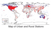
Moreover, the definition of urban areas is subject to some uncertainty, both in terms of how urban form is characterized and at what distance from built surfaces urban-related effects persist. Published station metadata often includes outdated indications of whether a station is urban or rural, and instrument geolocation data can be imprecise, out of date, or otherwise incorrect.

There is also uncertainty over how much explicit correction is needed for urban warming in global temperature reconstructions, and how well homogenization techniques recently introduced in GHCN-Monthly version 3 both detect and correct for inhomogenities arising from changes in urban form.

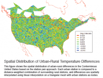
To address these issues and obtain a more accurate estimation of the impact of urbanization on land temperature trends, we examine different urbanity proxies at multiple spatial resolutions and urbanity selection criteria through both simple spatial weighting and station pairing techniques. This study limits itself to unadjusted average temperature data, though we will examine homogenized data in the future to see how much of the UHI signal is removed.

Methods

We examine GHCN-Daily version 2.80 temperature data rather than the more commonly used GHCN-Monthly data as it contains significantly more stations, particularly during the past thirty years, and allows for separate examination of maximum and minimum temperatures. A relatively high spatial density of stations is useful to allow sampling into various urban and rural station subsets while minimizing biases due to loss of spatial coverage. After excluding stations that have fewer than 36 months at any time in the period of record or at least one complete year of data during the 1979 to 2010 period, we are left with 14,789 stations.

A complete set of metadata is calculated for each station using the station location information provided in station inventories and publically available GIS datasets. These datasets include: Distance From Coast (0.1 deg), Hyde 3.1 historical population data (5arc minute), 2000AD Grump Population density (30 arc seconds), Grump Urban Extent, Land use classes from the Harmonized Land Use inventory (5 arc minutes), radiance calibrated Nightlights (30 arc seconds), ISA- Global Impervious Surfaces (30 arc seconds), Modis Landcover classes (15 arc seconds), and distance from the closest airport (30 arc seconds). In addition, area statistics at progressive radii are calculated around each putative site location.

Stations are then divided into two classes based on various thresholds for urbanity and two analytical methods are used to estimate the bias in trend due to urbanity: a spatial method and a paired station approach. The spatial averaging method relies on solving a set of linear equations for the stations in each class. For each group of stations, urban and rural, a time series of average temperature offsets was created by fitting the model:

where T represents the observed temperature for each station, month and year, L is a local average temperature for each station for each month (incorporating seasonal variation) and G is the desired global (or regional) average, varying by year. This is fitted with a weighting that is inversely proportional to a measure of station density. With a G calculated for both urban and rural, the trends can be compared.

The pairwise method proceeds with the same classification of stations and the following steps are taken. An urban base pair is selected based on the length of record. To qualify as a base urban pair a station must have 30 complete years of data in the 1979-2010 window.

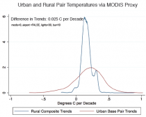
Ten out of 12 months of data are required to count as a complete year. For every urban base station rural pairs are selected based on distance and data overlap. For every urban base station the rural stations are exhaustively searched and all those rural pairs within 500km are assigned to the base station. Since rural stations may have short records the entire rural ensemble is evaluated for data overlap with the urban base pair. 300 months of overlap are required. If the collection of rural stations has less than 300 months of overlap with its urban pair, it is dropped from the analysis. A weighting function is deÞned in the neighborhood of each urban station, which diminishes with distance and is zero outside a certain radius. An average trend is computed for the rural stations within that radius by fitting the model where t is time in years, and B is the gradient. This trend is then compared with the OLS trend for the central urban station. The differences in the shapes of the distributions of the trends is a function of the number of stations that form the trend estimation.

Urban trends are trends for individual stations, while rural trends are the result of computing a trend for all the rural pairs taken as a complete ensemble.

Discussion

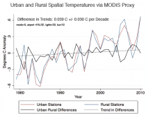
While urban warming is a real phenomenon, it is overweighted in land temperature reconstructions due to the oversampling of urban areas relative to their global land coverage. Rapid urbanization over the past three decades has likely contributed to a modest warm bias in unhomogenized global land temperature reconstructions, with urban stations warming about ten percent faster than rural stations in the period from 1979 to 2010. Urban stations are warming faster than rural stations on average across all urbanity proxies, cutoffs, and spatial resolutions examined, though the underlying data is noisy and there are many individual cases of urban cooling. Our estimate for the bias due to UHI in the land record is on the order of 0.03C per decade for urban stations.

This result is consistent with both the expected sign of the effect and regional estimates covering the same time period (Zhou et al 2004) and differs from some recent work suggesting zero or negative UHI bias (Wickham et al, submitted).

Stricter urbanity proxies that result in a smaller set of rural stations show larger urban-rural differences in trend. The upper limit on UHI bias between rural and urban stations is on the order of 0.06 to 0.1C per decade. However, these cases are clearly problematic from the spatial coverage aspect, as the number of rural stations becomes vanishingly small when the most stringent filters are applied. Adopting cutoffs that define rural less strictly leads to more reasonable spatial coverage and an estimate of UHI bias in the record that converges on 0.02C to 0.04C per decade across the proxies. The station pair approach avoids this issue by limiting the analysis to areas with both rural and urban stations available, but has limited global coverage and excludes large areas in India and coastal China where rapid urbanization has been occurring in recent decades.

It is likely that homogenization will further reduce the observed UHI-related bias, as many urbanity biases are detectable through break-point analysis via comparison to surrounding rural stations. We are currently in the process of using the Pairwise Homogenization Algorithm (Menne and Williams 2009) on GHCN-Daily data to examine the effects in more detail. However, it remains to be seen to what degree UHI bias can be removed via homogenization in areas like coastal China and India where there are few rural stations and where station densities are not particularly high in the current version of GHCN-Daily. In any case, the acquisition of additional station data outside of urban areas in these parts of the world would likely be benefitial.

Acquiring more accurate station location data will allow us to use higher-resolution remote sensing tools to identify urban characteristics below the 5 km threshold, and better test effects of site-specifc vs. meso-scale characteristics on urban warming biases. In addition, validated site locations allows for more refinement in the definition of rural stations as a function of distance from urban cores of various sizes.

References

Center for International Earth Science Information Network (CIESIN), Columbia University; International Food Policy Research Institute (IFPRI); The World Bank; and Centro Internacional de Agricultura Tropical (CIAT). 2004. Global Rural-Urban Mapping Project, Version 1 (GRUMPv1): Population Density Grid. Palisades, NY: Socioeconomic Data and Applications Center (SEDAC), Columbia University. Available at http://sedac.ciesin.columbia.edu/gpw.[Aug 14, 2011].

Elvidge, C.D., B.T. Tuttle, P.C. Sutton, K.E. Baugh, A.T. Howard, C. Milesi, B. Bhaduri, and R. Nemani, 2007, “Global distribution and density of constructed impervious surfaces”, Sensors, 7, 1962-1979

Fischer, G., F. Nachtergaele, S. Prieler, H.T. van Velthuizen, L. Verelst, D. Wiberg, 2008. Global Agro-ecological Zones Assessment for Agriculture (GAEZ 2008). IIASA, Laxenburg, Austria and FAO, Rome, Italy.

Klein Goldewijk, K. , A. Beusen, and P. Janssen (2010). Long term dynamic modeling of global population and built-up area in a spatially explicit way, HYDE 3 .1. The Holocene20(4):565-573.

Klotzbach, P., R. Pielke Sr., R. Pielke Jr., J. Christy, and R. T. McNider, 2009. An alternative explanation for differential temperature trends at the surface and in the lower troposphere. J. Geophys. Res.

Menne, M.J., I. Durre, R.S. Vose, B.E. Gleason, and T.G. Houston, 2011: An overview of the Global Historical Climatology Network Daily Database. Journal of Atmospheric and Oceanic Technology, submitted.

Menne, M.J., and C.N. Williams, Jr., 2009. Homogenization of temperature series via pairwise comparisons. J. Climate, 22, 1700-1717.

Schneider, A., M. A. Friedl and D. Potere (2009) A new map of global urban extent from MODIS data. Environmental Research Letters, volume 4, article 044003.

Schneider, A., M. A. Friedl and D. Potere (2010) Monitoring urban areas globally using MODIS 500m data: New methods and datasets based on urban ecoregions. Remote Sensing of Environment, vol. 114, p. 1733-1746.

T. R. Oke (1982). “The energetic basis of the urban heat island”. Quarterly Journal of the Royal Meteorological Society 108: 1–24.

Wickham, C., J. Curry, D Groom, R. Jacobsen, R. Muller, S. Perlmutter, R. Rohde, A. Rosenfeld, and J. Wurtele, 2011. Inßuence of Urban Heating on the Global Temperature Land Average Using Rural Sites IdentiÞed from MODIS ClassiÞcations.

Submitted.

Zhou, L., R. Dickinson, Y. Tian, J. Fang, Q. Li, R. Kaufmann, C. Tucker, and R. Myneni, 2004. Evidence for a significant urbanization effect on climate in China. Proceedings of the National Academy of Sciences.

Ziskin, D., K. Baugh, F. Chi Hsu, T. Ghosh, and C. Elvidge, 2010, “Methods Used For the 2006 Radiance Lights”, Proceedings of the 30th Asia-Pacific Advanced Network Meeting, 131-142