Feb 14, 2011
Why Wind Won’t Work
Submission to Australian Senate Enquiry by Viv Forbes, Carbon Sense Coalition
Here is an excellent summary of all the issues with wind power, why it hasn’t worked and won’t work for meeting future energy needs and why environmentalists and politicians push it despite that fact to achieve other agendas. It is a must read.
Why are governments still mollycoddling wind power?
There is no proof that wind farms reduce carbon dioxide emissions and it is ludicrous to believe that a few windmills in Australia are going to improve global climate.
Such wondrous expressions of green faith put our politicians on par with those who believe in the tooth fairy.
The wind is free but wind power is far from it. Its cost is far above all conventional methods of generating electricity.
Tax payers funding this “Wind Welfare” and consumers paying the escalating power bills are entitled to demand proof.
Not only is there no climate justification for wind farms, but they are also incapable of supplying reliable or economical power.
It is also surprising those who claim to be defenders of the environment can support this monstrous desecration of the environment.

Wind power is so dilute that to collect a significant quantity of wind energy will always require thousands of gigantic towers each with a massive concrete base and a network of interconnecting heavy duty roads and transmission lines. It has a huge land footprint.
Then the operating characteristics of turbine and generator mean that only a small part of the wind’s energy can be captured.
Finally, when they go into production, wind turbines slice up bats and eagles, disturb neighbours, endanger health, reduce property values and start bushfires.
Wind power is intermittent, unreliable and hard to predict. To cover the total loss of power when the wind drops or blows too hard, every wind farm needs a conventional back-up power station (commonly gas-fired) with capacity of twice the design capacity of the wind farm to even out the sudden fluctuations in the electricity grid. This adds to the capital and operating costs and increases the instability of the network.
Why bother with the wind farm - just build the backup and achieve lower costs and better reliability?
There is no justification for continuing the complex network of state and federal subsidies, mandates and tax breaks that currently underpin construction of wind farms in Australia. If wind power is sustainable it will be developed without these financial crutches.
Wind power should compete on an equal basis with all other electricity generation options.
Europe Pulling the Plug on Green Energy Subsidies
“The Spanish and Germans are doing it. So are the French. The British might have to do it. Austerity-whacked Europe is rolling back subsidies for renewable energy as economic sanity makes a tentative comeback. Green energy is becoming unaffordable and may cost as many jobs as it creates.
But the real victims are the investors who bought into the dream of endless, clean energy financed by the taxpayer. They forgot that governments often change their minds.” Eric Reguly, The Globe and Mail, 27 Jan 2011. Reported in CCNet 28 Jan 2011.
See the full report and copy and distribute to friends and family. It should make you and them rethink wind as a solution and start objecting to those in power who push it.
Feb 12, 2011
Cap-trade issue heats up hearing
By Kevin Landrigan, Nashua Telegraph
A legislative bid for New Hampshire to pull out of a 10-state, regional greenhouse gas initiative turned into an ideological war Thursday over the credibility of the science of climate change.
But Gov. John Lynch tried to steer the debate to one of dollars and cents, warning that repeal of the 3-year-old law would hit businesses and consumers in the wallet.
“Withdrawing from RGGI would be a blow to our economy and to our state’s efforts to become more energy efficient and energy independent,” Lynch wrote to the House Science Technology and Energy Committee, which hosted an all-day hearing on the repeal bill (HB 519) in Representatives Hall.
New Hampshire became the last of the states in the region to sign onto RGGI, which makes polluters buy allowances for carbon dioxide emissions that studies show contribute to greenhouse gases.
Jessica O’Hare, program associated at Environment New Hampshire, said this form of cap-and-trade encourages businesses to change New Hampshire’s status as one of the top five states in consumption of oil per capita. “It helps New Hampshire reduce our reliance on oil and other fossil fuels,” O’Heare said. “This will make the state more economically secure and reduce pollution.”
Joseph D’Aleo, a Hudson meterologist and climatologist said CO2 is not a pollutant but a beneficial gas and these programs have no measurable effect on climate. “RGGI represents the epitome of all-pain-and-no-gain scenario,” D’Aleo said.
Eric Werme, a Boscawen software engineer and climate enthusiast, agreed and said ocean currents have had much more to do with affecting climate and warming of the planet than any man-made program to encourage reduction of emissions.
“I consider it premature for government to try and influence any restriction on CO2 emissions at this point,” Werme said.
But Kenneth Colburn of Stonyfield Farm Yogurt in Londonderry, said the program has already led to $21 million worth of energy efficiencies and 1,130 jobs. Repeal of the program would hurt the state economically, he warned. “This will increase costs on New Hampshire businesses and citizens and provide them with no accompanying benefit whatsoever,” said Colburn, a former state director of air resources.
“This is hardly the New Hampshire way, and would detract from rather than contribute to the New Hampshire advantage.” Lynch maintained since RGGI began, it has cost consumers $11 million and delivered $28 million in benefits.
Current Air Resources Director David Scott said RGGI is a modest program that encourages and does not punish businesses regarding their emissions.
“RGGI was never meant to solve the climate change issue; it was meant to be a modest, unique program and it has been,” Scott added. Post here.
Icecap Note: with required purchase of allowances the costs for electricity/energy prices rise, which has a ripple effect, translating into higher costs for manufacturing and transportation and for running retail and service business and thus higher costs for all goods and services. That is a stealth tax. Like in the Federal Goverenment, the ‘benefits’ go to inflated bureaucracies and subsidized industries - like alternative energy and energy efficiency corporations. The state does not need to tax indiustry and consumers to provide these businesses relief, just reduce their tax liability. If their businesses make sense, they will survive. In many of the other states in the northeast under RGGI, money from allowances goes into the general fund, to fund state business and reduce huge deficits. It is on top of state taxes. Attached are the two presentations submitted to the committee here and here. Here was a great introductory statement by Andrew Manuse, a legislator to the committee.
The Bangor Daily news reported NH last year raided the funds to help pay for other state spending. They are not alone. You can’t trust bureacrats to spend tax dollars wisely or as they originally promised.
Feb 10, 2011
Clean Energy Standard: Cap-and-Trade Only Less Efficient
By Marlo Lewis, GlobalWarming.org
As noted previously on GlobalWarming.Org, Obama’s “Clean Energy Standard” would effectively impose the Waxman-Markey cap-and-trade bill’s emission reduction target on the electric power sector.
Under Obama’s proposal, “By 2035, 80% of America’s electricity will come from clean energy sources” (i.e. from wind, solar, hydro, nuclear, “clean coal,” and natural gas). Similarly, an estimated 81% of U.S. electricity would come from such sources in 2030 in the Energy Information Administration’s “Basic Case” analysis of the Waxman-Markey bill.
There is one difference though. Emission reductions accomplished via Soviet-style production quota (mandates) such as a clean energy standard would likely be more costly than emission reductions accomplished via market-like mechanisms such as cap-and-trade. National Journal reporter Amy Harder spotted this issue last Friday:
“One of the things that happens implicitly when you set a standard is that you have in fact put a price on carbon, but it’s the clumsiest way to do it,” said Kevin Book, managing director at ClearView Energy Partners, an energy consulting company. “You’re not looking for an efficient, market-based solution. You’re looking for just enough to meet the standards solution.”
Get the picture? The public rejected cap-and-trade, punishing at the polls several Members of Congress who voted for Waxman-Markey. Instead of abandoning a policy designed to make our electric rates “necessarily skyrocket,” Obama offers a more costly version of the same agenda.
Cap-and-trade is dead because the public finally caught on that it is a stealth energy tax, a big reason being that it makes coal - the most economic electricity fuel in many markets - uncompetitive. Coal generated 44.5% of all U.S. electricity and almost 64% of U.S. baseload power in 2009, according to the U.S. Energy Information Administration (EIA).
Obama’s clean energy standard too would make coal generation uneconomic. “Clean” essentially means “anything but coal.” Instead of pricing the carbon emissions from coal, as a cap-and-trade program does, Obama’s new policy would simply prohibit “conventional coal” from competing with other energy sources in 80% of the nation’s electricity market. Existing coal plants could continue to operate within the 20% segment that is deemed “unclean” - unless, of course, EPA’s war on coal succeeds in forcing those plants into premature retirement.
Unless CCS gets a whole lot cheaper soon, Obama’s clean energy standard will effectively ban the construction of new coal-fired power plants. That is a long-standing goal of the Sierra Club and other eco-litigation groups. However, it is emphatically not what either major party campaigned for in last year’s congressional races.
On the day after Election Day, Obama told the Washington press corps: “Cap and trade was just one way of skinning the cat; it was not the only way. It was a means, not an end. And I’m going to be looking for other means to address this problem.” Obama’s proposed clean energy standard would skin the cat known as the American ratepayer every bit as much - and perhaps more - than cap-and-trade.
See full post.
Feb 10, 2011
Orwellism of the Day: Bulb Ban Is Freedom
By Henry Payne
In a leap of Orwellian logic, USA Today - America’s second-largest newspaper argued in its lead editorial Tuesday that banning the incandescent light bulb is a victory for free markets.
“The best way for government to boost energy efficiency isn’t to micromanage by picking winners and losers, a job better suited to free-market innovation. It is to set a reasonable standard - miles per gallon or light per watt, for example - and let the market sort it out,” spins the editorial in support of picking winners and losers.” That’s what Congress did in 2007 “in banning the bulb”.
War is Peace. Freedom is Slavery. Ignorance is Strength. Banning is choice. Regulation is freedom.
One wonders if USA Today’s editors would tolerate this doublethink if applied to their own industry. Were Congress to ban newspapers in order to force them onto the more “planet-friendly” Internet, would USA Today swallow this as free-market economics?
Michigan View contributor Ted Nugent quipped that “Obama slept through the election” after a State of the Union address that stubbornly plowed ahead with the hyper-regulation of carbon and Big Government spending. Obama’s MSM allies were apparently snoozing on the couch next to him.
Or perhaps Obamedia is very awake. And they realize that - given the unpopularity of their radical green agenda — the only way to move if forward is with Newspeak that would make Big Brother blush.
Read more at the Michigan View.com.
Feb 08, 2011
In reply to “The Importance of Science in Addressing Climate Change”
CO2Science and 68 signatories
To the Members of the U.S. House of Representatives and the U.S. Senate:
February 8, 2011
In reply to “The Importance of Science in Addressing Climate Change”
On 28 January 2011, eighteen scientists sent a letter to members of the U.S. House of Representatives and the U.S. Senate urging them to “take a fresh look at climate change.” Their intent, apparently, was to disparage the views of scientists who disagree with their contention that continued business-as-usual increases in carbon dioxide (CO2) emissions produced from the burning of coal, gas, and oil will lead to a host of cataclysmic climate-related problems.
We, the undersigned, totally disagree with them and would like to take this opportunity to briefly state our side of the story.
The eighteen climate alarmists (as we refer to them, not derogatorily, but simply because they view themselves as “sounding the alarm” about so many things climatic) state that the people of the world “need to prepare for massive flooding from the extreme storms of the sort being experienced with increasing frequency,” as well as the “direct health impacts from heat waves” and “climate-sensitive infectious diseases,” among a number of other devastating phenomena. And they say that “no research results have produced any evidence that challenges the overall scientific understanding of what is happening to our planet’s climate,” which is understood to mean their view of what is happening to Earth’s climate.
To these statements, however, we take great exception. It is the eighteen climate alarmists who appear to be unaware of “what is happening to our planet’s climate,” as well as the vast amount of research that has produced that knowledge.
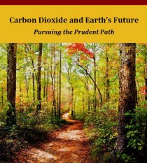
For example, a lengthy review of their claims and others that climate alarmists frequently make can be found on the Web site of the Center for the Study of Carbon Dioxide and Global Change (see Carbon Dioxide and Earth’s Future: Pursuing the Prudent Path). That report offers a point-by-point rebuttal of all of the claims of the “group of eighteen,” citing in every case peer-reviewed scientific research on the actual effects of climate change during the past several decades.
If the “group of eighteen” pleads ignorance of this information due to its very recent posting, then we call their attention to an even larger and more comprehensive report published in 2009, Climate Change Reconsidered: The 2009 Report of the Nongovernmental International Panel on Climate Change (NIPCC). That document has been posted for more than a year in its entirety at www.nipccreport.org.
These are just two recent compilations of scientific research among many we could cite. Do the 678 scientific studies referenced in the CO2 Science document, or the thousands of studies cited in the NIPCC report, provide real-world evidence (as opposed to theoretical climate model predictions) for global warming-induced increases in the worldwide number and severity of floods? No. In the global number and severity of droughts? No. In the number and severity of hurricanes and other storms? No.
Do they provide any real-world evidence of Earth’s seas inundating coastal lowlands around the globe? No. Increased human mortality? No. Plant and animal extinctions? No. Declining vegetative productivity? No. More frequent and deadly coral bleaching? No. Marine life dissolving away in acidified oceans? No.
Quite to the contrary, in fact, these reports provide extensive empirical evidence that these things are not happening. And in many of these areas, the referenced papers report finding just the opposite response to global warming, i.e., biosphere-friendly effects of rising temperatures and rising CO2 levels.
In light of the profusion of actual observations of the workings of the real world showing little or no negative effects of the modest warming of the second half of the twentieth century, and indeed growing evidence of positive effects, we find it incomprehensible that the eighteen climate alarmists could suggest something so far removed from the truth as their claim that no research results have produced any evidence that challenges their view of what is happening to Earth’s climate and weather.
But don’t take our word for it. Read the two reports yourselves. And then make up your own minds about the matter. Don’t be intimidated by false claims of “scientific consensus” or “overwhelming proof.” These are not scientific arguments and they are simply not true.
Like the eighteen climate alarmists, we urge you to take a fresh look at climate change. We believe you will find that it is not the horrendous environmental threat they and others have made it out to be, and that they have consistently exaggerated the negative effects of global warming on the U.S. economy, national security, and public health, when such effects may well be small to negligible.
See this PDF with the 68 signatories.
|